

Relative Price Shocks and Inflation: The Role of Monetary Policy
Key Takeaways
- "Relative price shocks" — or shocks to supply and demand for particular categories of consumption — can move the inflation rate.
- The effect of relative price shocks on inflation depends critically on monetary policy.
- The effect of relative price shocks on inflation is temporary unless monetary policy makes it permanent.
The implications of artificial intelligence (AI) for inflation are currently a source of much attention. Some commentators have suggested AI may affect inflation through an increase in the demand for, and thus the price of, components used in consumer electronics.
This is far from the only time that there have been discussions involving connections between price changes for particular items and overall inflation. In the spring of 2021, for example, used car prices rose 25 percent in just three months. And energy and food prices can be so volatile that economists and policymakers often look at inflation measurements that exclude them (called "core" inflation).
In principle, changes in the supply and demand conditions for specific goods could affect mainly their relative prices, with little in the way of implications for inflation. Yet in reality, there do seem to be connections between some relative price changes and the overall inflation rate. The use of core inflation measures is because inflation tends to be correlated with relative price changes for gasoline.
More generally, my 2024 working paper "The Relationship Between Inflation and the Distribution of Relative Price Changes" — co-authored with Andreas Hornstein and Francisco Ruge-Murcia — shows that the period 1995-2019 exhibited a close relationship between the monthly inflation rate and the share of relative price increases (which is a summary statistic for the distribution of relative price changes). We showed that inflation tended to be high or low relative to its average level depending on whether the share of relative price increases was low or high. The meaning of a low share of relative price increases is that a small share of expenditure is on goods and services with especially large relative price increases, while a large share of expenditure is on categories of goods and services whose relative price falls. This happens, for example, when there is a large increase in the price of gasoline.
This article uses an economic model featuring multiple categories of consumption goods to illustrate three points:
- "Relative price shocks" — or shocks to supply and demand for particular categories of consumption — can move the inflation rate.
- The effect of relative price shocks on inflation depends critically on monetary policy.
- The effect of relative price shocks on inflation is temporary unless monetary policy makes it permanent.
Any statements about the effects of AI on inflation are implicitly (or explicitly) making assumptions about the behavior of monetary policy. While our focus is on the relative price shocks channel, the dependence on monetary policy also applies to other channels through which AI could affect inflation.
Background on Inflation and Relative Price Changes
Inflation
The Federal Open Market Committee targets a 2 percent inflation rate for the personal consumption expenditures (PCE) price index. The PCE inflation rate is roughly equal to a weighted average of the price changes for more than 200 consumption categories, where each category's weight is equal to its expenditure share in the previous month.1
Relative Price Changes
For each of the items that contribute to the PCE inflation rate, we call their actual price change a nominal price change, because it is measured in unadjusted dollars. The relative price change for each item is the difference between the nominal price change and the PCE inflation rate.
The definition of a relative price change implies that the average relative price change across all items comprising the price index is zero. To see this, observe that the average relative price change is the difference between the average nominal price change and the inflation rate, which itself is equal to the average nominal price change. Figure 1 plots the 12-month relative price changes for durable goods, nondurable goods and services — which are the three broadest PCE categories — for 1995 to the present. The expenditure shares are approximately 10 percent for durables, 20 percent for nondurables and 70 percent for services.
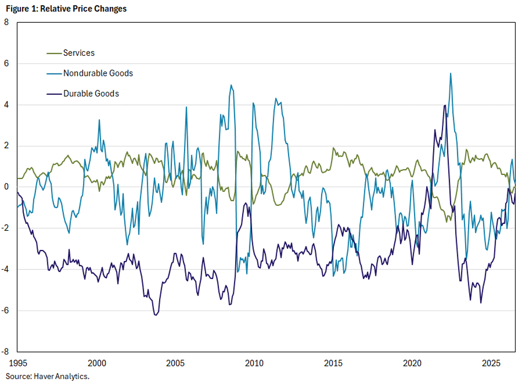
The average relative price change is zero no matter how the distribution of relative price changes behaves: The distribution varies across time in Figure 1, but the average is always zero. It follows that there is no necessary relationship between the distribution of relative price changes and the inflation rate. For example, imagine a scenario where the relative price of gasoline doubles. (Note that the expenditure share of gasoline is about 2 percent.)
- One way the relative price of gasoline could double (rise by 100 percent) is for its nominal price to rise 102 percent, all other prices to fall slightly and the inflation rate to be 2 percent.
- Another way the relative price of gasoline could double is for its nominal price to rise by more than 104 percent and all other prices to rise by 2 percent, yielding an inflation rate of just above 4 percent.
If the shock were to occur in an otherwise stable situation — with inflation near the Fed's 2 percent target — the second scenario intuitively seems more likely than the first: Other prices would behave as before instead of immediately falling in reaction to the shock to keep inflation at target. (Of course, it's a gross simplification to assume that all other prices rise at 2 percent.)
As mentioned above, there is empirical evidence of a relationship between the distribution of relative price changes and inflation. And the example just given provides suggestive intuition for why what we call relative price shocks would move inflation. An economic model can be used to illustrate these points and investigate further.
Model Description
The model is taken from an updated version of my 2022 working paper "Relative Price Shocks and Inflation," co-authored with Francisco Ruge-Murcia. It is a multisector New Keynesian model in which there are shocks to supply and demand in each of 15 sectors. There is an input-output structure which allows shocks to supply or demand in one sector to have spillover effects in other sectors. Monetary policy is assumed to follow a simple Taylor-style rule, where the interest rate depends on its lagged value and the behavior of inflation and output. And monetary policy matters for the real economy as well as inflation because nominal prices are costly to adjust.2 The model's parameters are estimated using U.S. data on sectoral prices and quantities from January 1995 to February 2020.
To illustrate the points mentioned at the outset, this article will discuss the model economy's response to a persistent negative shock to productivity in the production of "recreational goods," which is the PCE category that includes personal computers and peripheral equipment.
It may seem odd to talk about a negative productivity shock for computer production in the context of AI, but this is a crude approximation. A richer model would study a positive broad-based shock to anticipated productivity that triggered massive investment requiring computer chips. In turn, because those chips are also inputs into personal computers, the cost of producing computers would go up. Thus, the exogenous positive AI productivity shock would endogenously increase price and decrease the quantity of consumer products using semiconductors.
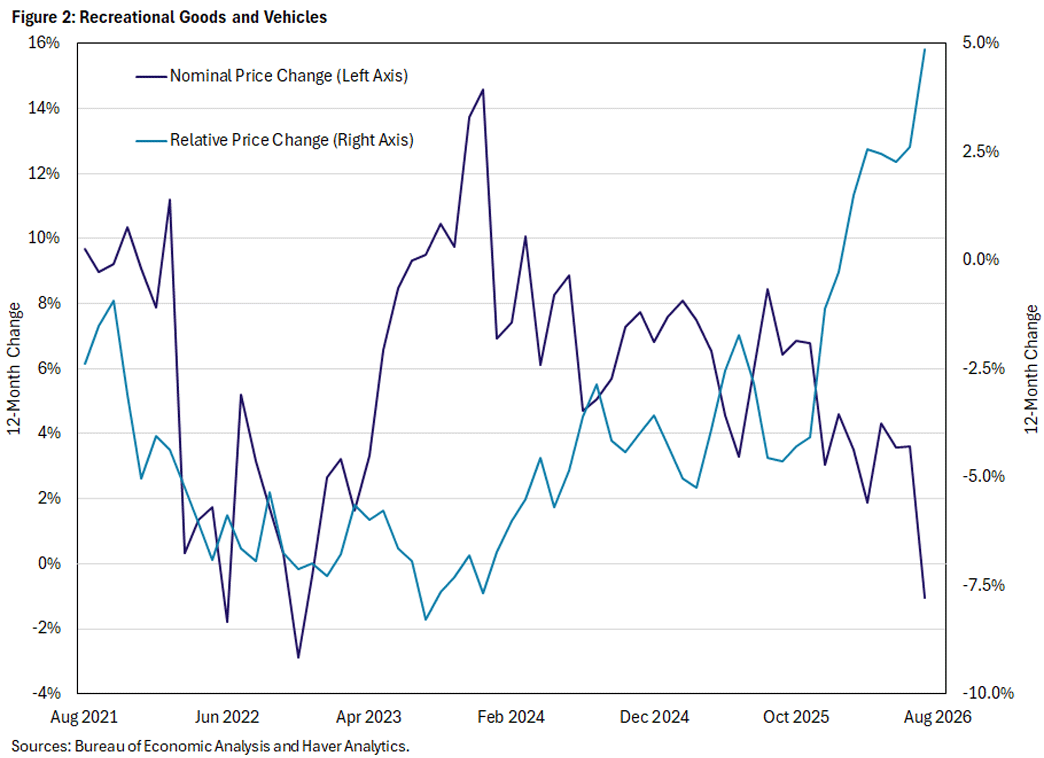
The best way to approximate that scenario in the model is with a negative productivity shock for recreational goods-producing firms, as that shock will raise the price and reduce the quantity of recreational goods. As shown in Figure 2, a price increase and quantity decrease is what we have seen in the data.
Results From the Model
Figures 3, 4 and 5 plot the response of selected model variables to a negative productivity shock hitting the recreational goods and vehicles sector. The shock is large, as it is calibrated so that the relative price of the goods produced by that sector rises by about 25 percent in the month of impact. That calibration assumes monetary policy is given by the estimated monetary policy rule, with a coefficient on inflation of 1.5. It also compares outcomes under alternative policy rules with much lower (1.01) and higher (10) values of the coefficient on inflation.
Relative Price Changes
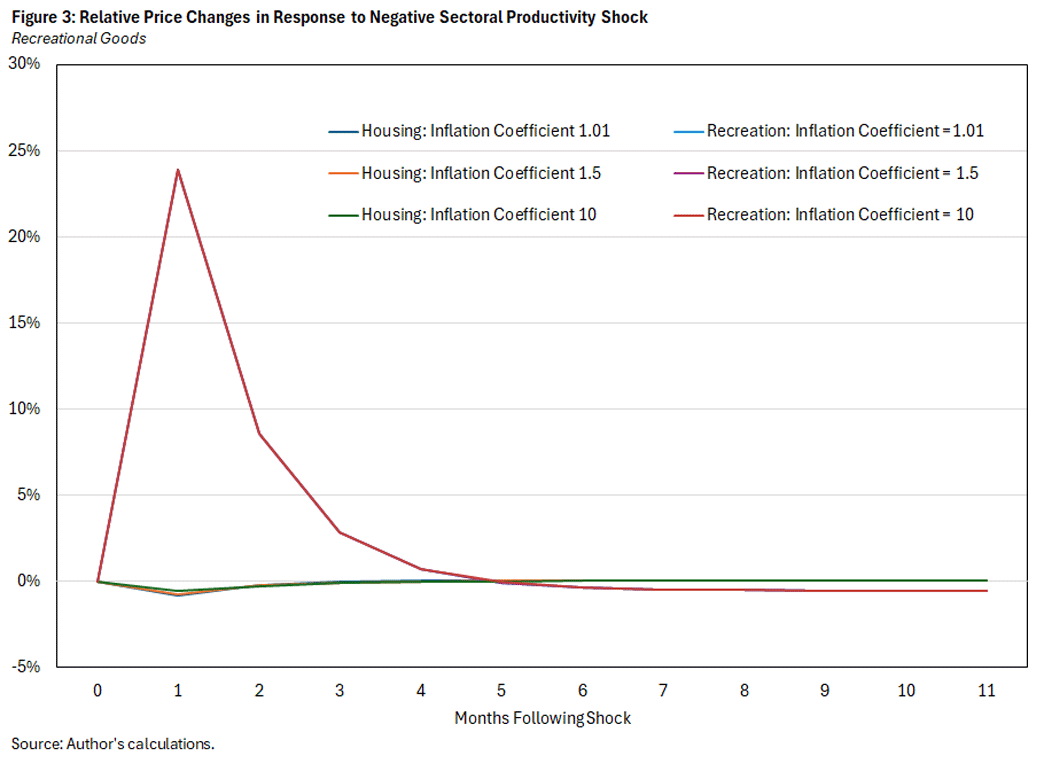
Figure 3 plots the relative price changes both for the goods produced by the category hit by the shock (recreation) and for housing and utilities services. I chose housing because it is a large share of consumption (about 18 percent).
Figure 3 shows that these relative price changes are largely invariant to the monetary policy rule. In each case, the relative price of recreational goods rises by 24 percent and then falls back to its balanced growth path, which involves a gradual decrease. In contrast, the relative price of housing and utilities barely moves in response to this shock: It falls slightly before moving back up to its gradually increasing balanced growth path. The relative price responses in Figure 3 provide some justification for referring to the shock as a relative price shock, although relative prices do depend to some degree on the behavior of policy.
Inflation
Based on Figure 3, one might think that the policy rule is irrelevant for the response of the economy to this large shock to one sector. However, recall from above that the behavior of relative prices need not tell us anything about the behavior of nominal prices. And indeed, Figure 4 shows that the inflation rate behaves quite differently for each of the policy rules. In the benchmark case, with the policy rule coefficient on inflation of 1.5, monthly inflation shoots up from 2 percent to almost 10 percent annualized on impact. Inflation then falls to 4 percent the next month and dips slightly below 2 percent after five months before smoothly converging back to target.
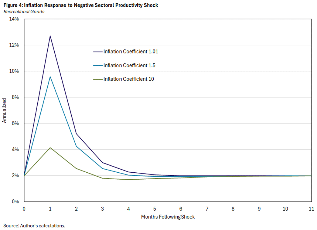
Increasing the interest rate rule coefficient on inflation to 10 reduces the impact response of inflation by more than half, as it rises from 2 percent before the shock to 4.1 percent on impact before falling to 1.8 percent in the third month. Conversely, a very small coefficient on inflation (1.01) results in the inflation rate rising to 12.7 percent on impact and returning to steady state only after six months.
Nominal Sectoral Price Changes
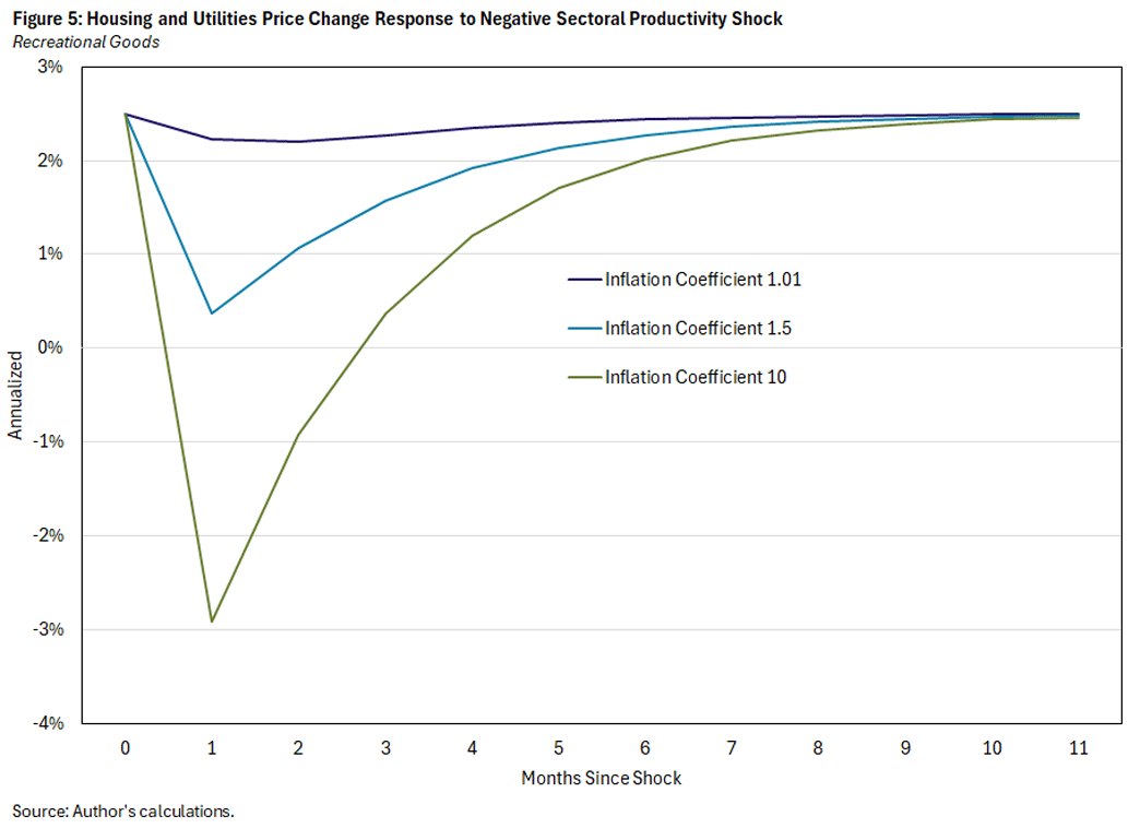
With relative price changes being nearly invariant to the policy rule and inflation being sensitive to the policy rule, it follows that the nominal price changes for each consumption category are sensitive to the policy rule. I only show housing in Figure 5 because the annualized nominal price changes for recreational goods are so large: The 24 percent monthly relative price change translates to more than 1,200 percent at an annual rate.
Before the shock hits and after it has faded, the nominal price of housing services rises at about a 2.5 percent annual rate. On impact, housing services prices rise at about a 0.5 percent annual rate for the benchmark policy setting. When the policy rule coefficient on inflation is 10 — which comes close to stabilizing overall inflation — housing services prices fall by 3 percent at an annualized rate. And finally, when the policy rule has a low coefficient on inflation (1.01), housing services prices barely move in response to the shock.
Takeaways
I began the analysis with a discussion of AI and the price of semiconductors. But the analysis applies to any shock that causes a relative price change large enough that if all other prices behaved as normal, there would be a noticeable effect on inflation. The magnitude of the shock examined here was purposely extreme, but qualitatively the results are instructive:
- A large sectoral shock has a large effect on relative prices regardless of the policy rule, although in the short run the magnitude of the relative price response is not entirely invariant to the policy rule.
- For a benchmark policy rule, the inflation rate responds strongly to the relative price shock in the same direction as the relative price for the category hit by the shock. Different policy rule parameters correspond to much smaller or larger responses of inflation, though the inflation response is temporary in each case.
- A policy rule that stabilizes inflation in response to the shock results in a large decrease in the price of housing services in the impact period of the shock. In contrast, there is little change in housing services prices (relative to their average increase) if the policy rule allows maximal pass through to inflation from the shock. Though not shown, the same qualitative results apply for other categories: Stabilization of inflation requires large offsetting price decreases for the categories not hit by the shock.
Stepping away from the model, it seems unrealistic that, in response to a large shock that raises the relative price for one category of consumption, other prices would fall such that inflation would be stable. It seems more likely that other prices would continue with their typical behavior, such that the price increase for the affected category would fully pass through to inflation. This presents a bit of a conundrum, since the policy rule that results in full passthrough involves a much lower coefficient on inflation than in the estimated model.
The resolution likely involves (in part) monetary policy following a more complicated rule than assumed here: In response to typical fluctuations in the economy, policy may be well characterized by a rule with an inflation coefficient of 1.5. But when there are large relative price shocks, policy lets them pass through to inflation, avoiding the requirement for large offsetting changes in the prices of other consumption categories. The model also makes the simplifying assumption that firms and consumers have perfect information about the shocks hitting the economy. In practice, slow information diffusion may be one factor that leads firms to continue with their typical behavior in response to shocks to other sectors.
Alexander L. Wolman is vice president for monetary and macroeconomic research in the Research Department at the Federal Reserve Bank of Richmond.
For more information on the PCE price index — including the exact formula — see the 1999 article "A Comparison of the CPI and the PCE Price Index (PDF)" by Todd Clark.
The model specifies price stickiness as in the 1982 paper "Sticky Prices in the United States" by Julio Rotemberg.
To cite this Economic Brief, please use the following format: Wolman, Alexander L. (November 2026) "Relative Price Shocks and Inflation: The Role of Monetary Policy." Federal Reserve Bank of Richmond Economic Brief, No. 26-38.
This article may be photocopied or reprinted in its entirety. Please credit the author, source, and the Federal Reserve Bank of Richmond and include the italicized statement below.
Views expressed in this article are those of the author and not necessarily those of the Federal Reserve Bank of Richmond or the Federal Reserve System.


Receive a notification when Economic Brief is posted online.