Estimating Aggregate Fiscal Multipliers from Local Data
Variations among regions in their responses to economic policies can be used to estimate the effects of those policies at the national level while minimizing or eliminating issues of reverse causation. Recent research has employed county-level data to look at the effects of federal government spending — in particular, the 2009–12 stimulus — on aggregate consumption.
Even though all, or nearly all, students of introductory macroeconomics are taught about the Keynesian multiplier, there is surprisingly little consensus on just what the numeric value of the multiplier is. The literature has yielded a range of estimates of both the consumption multiplier (that is, the effect of a one-dollar increase in government spending on private consumption spending) and the output multiplier (the effect on output). Indeed, there is not even full consensus on whether the consumption multiplier is positive or negative.
In recent research, Bill Dupor of the St. Louis Fed, Marios Karabarbounis of the Richmond Fed, Marianna Kudlyak of the San Francisco Fed, and M. Saif Mehkari of the University of Richmond have studied the consumption multiplier using a new approach that relies on local consumer spending data coupled with data on local public spending under the American Recovery and Reinvestment Act of 2009, or ARRA, as well as a structural model with rich heterogeneity that translates the regional consumption responses into an aggregate consumption response.1
Looking at Local Multipliers
The conventional approach to estimating a government spending multiplier is to analyze variations in aggregate consumption or output over time in relation to variations in government spending over time. Such an approach involves several challenges for researchers: (1) dealing with possible reverse causation (that is, changes in consumption or output may drive changes in government spending); (2) taking into account that consumption or output may respond to changing expectations about government spending, not just actual changes in government spending; and (3) isolating effects of fiscal policy changes from those of changes in monetary policy that may be taking place at the same time. Various methods have been developed to overcome these challenges. For instance, Valerie Ramey of the University of California, San Diego has introduced a methodology based on analysis of news texts to capture changes in expectations about spending, specifically military spending.2
An alternative approach to estimating multipliers looks not at aggregate variations over time, but instead at variations across regions. That is, the analysis considers how a one-dollar change in federal government spending within a region affects local consumption or output relative to regions that did not receive this change in spending. Estimates of the local multipliers are then aggregated into an estimate of the multiplier at the national level. Advantages of this approach include the availability of more data points and the availability of additional options for managing problems of reverse causation.
One such study is that of Emi Nakamura and Jón Steinsson of Columbia University, who estimated the output multiplier by looking at state-level changes in military expenditures, which vary considerably among states during military buildups and drawdowns.3 Their methodology addresses the problem of reverse causation in that military buildups and drawdowns are assumed not to be caused by economic downturns or upturns in specific states. Another study, by Sylvain Leduc and Daniel Wilson of the San Francisco Fed, looked at state-level changes in federal highway spending — again, on the basis that variations in those changes across states are not related to a state's current economic condition.4
Estimating Local Multipliers with Transaction Data
To estimate the consumption multiplier, Dupor, Karabarbounis, Kudlyak, and Mehkari use regional variations in federal spending under ARRA from 2009 through 2012 in combination with household data. Enacted during the Great Recession, ARRA provided approximately $840 billion in fiscal stimulus, including $228 billion in public contracts, grants, and loans. These contracts, grants, and loans were made or entered into by multiple agencies, including the Federal Highway Administration, the Department of Education, and the Department of Housing and Urban Development, among others.
Dupor, Karabarbounis, Kudlyak, and Mehkari take advantage of the fact that the federal government collected detailed information from recipients of ARRA funds and made it available on a public website, recovery.gov. Data available on each expenditure include the amount spent, the award date, and the zip code of the recipient. Where an award passed through multiple levels — for example, if an award was made by a federal agency to a state agency, which then turned the money over to private organizations — the data include information on the private organizations that ultimately spent the money. Thus, the researchers are able to tie the federal funds to the locales in which those organizations were based.
To avoid the possibility of reverse causation, where local economic conditions influenced the federal spending, the researchers include only the ARRA spending that was determined independently of those conditions (that is, was determined exogenously). They analyze the statute, regulations, and other guidance from the federal agencies to determine which spending met that standard. For example, Department of Education grants for children with disabilities flowed to a locality solely on the basis of the number of children with disabilities, not on the basis of local economic conditions. Highway maintenance grants, similarly, were made independently of economic conditions. By going through programs in this manner, the researchers identify approximately $46 billion in exogenous ARRA spending, or 20.2 percent of the total.
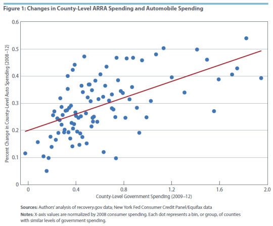
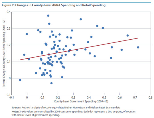
For data on local consumer spending at the zip code level, the researchers use information on retail spending from the Nielsen HomeScan dataset of 60,000 households and the Nielsen Retail Scanner dataset of 40,000 stores as well as information on auto loans from the New York Fed Consumer Credit Panel/Equifax dataset of 10 million individuals. The determination of local consumer spending with micro-level datasets, which is novel in the literature on the fiscal multiplier, allows for a finer level of geographic detail (and thus more observations) than in past work and is less vulnerable to measurement error.
Examining the response of local consumer spending to local changes in exogenous federal spending under ARRA, Dupor, Karabarbounis, Kudlyak, and Mehkari find that the response to fiscal stimulus is positive. (See Figures 1 and 2.) In particular, they estimate that a one-dollar increase in federal spending within a county increases local auto spending by an average of seven cents and local retail spending by an average of eleven cents. Overall, they estimate that a one-dollar increase in spending increases consumer spending within a county by an average of eighteen cents.
From Local Multipliers to an Aggregate Multiplier
The local multiplier — the fiscal multiplier identified from regional variations — represents the change in a macroeconomic variable (such as consumer spending or output) in one region relative to other regions that did not receive any government aid. The more familiar aggregate fiscal multiplier, in turn, is the total change in a macroeconomic variable (across all regions) in response to the total change in government spending.
The local multiplier would be expected to differ from the aggregate multiplier for a number of reasons. First, fiscal policy may lead to transfers from one region to another in the form of uneven spending (net of tax revenues) among regions. In the case of a one-dollar transfer from households in region A to households in region B, the full increase in consumer spending in region B would be reflected in the local multiplier for that region — but at the aggregate level, the net increase (if any) in spending would be less because there would be partially offsetting negative effects on spending in region A. Second, to the extent that regions trade with one another, federal spending increases in one region may be reflected in other regions. For example, consumers in a region where greater fiscal stimulus has occurred may buy more goods originating in other regions. This effect would tend to push the local multiplier lower than the aggregate multiplier. Third, monetary policy may lead to spillovers across regions; fiscal stimulus that is high enough in some regions to bring about inflation may lead the central bank to adopt a contractionary monetary policy that affects all regions, including those receiving fiscal stimulus and those not receiving it.5
To translate the local fiscal multiplier into an aggregate multiplier, the researchers use a structural model consisting of multiple regions, with each region consisting of many households that differ in terms of their market wages and asset holdings. In the model, higher public spending in a locality leads to more demand for local products and thus higher local prices and wages. Consequently, in the model, consumption rises, especially on the part of households with little wealth, which tend to have a higher marginal propensity to consume (that is, they tend to devote a larger share of new additional dollars to consumer spending). On the basis of this model, the researchers estimate an aggregate consumption multiplier of 0.4, roughly twice their estimate of the average local multiplier.
Bill Dupor is an assistant vice president in the Research Division of the St. Louis Fed, Marianna Kudlyak is a research advisor in the Economic Research Department at the San Francisco Fed, M. Saif Mehkari is an associate professor in the Economics Department at the University of Richmond, and Marios Karabarbounis is an economist and David A. Price is senior editor in the Research Department at the Richmond Fed.
Bill Dupor, Marios Karabarbounis, Marianna Kudlyak, and M. Saif Mehkari, "Regional Consumption Responses and the Aggregate Fiscal Multiplier," Federal Reserve Bank of Richmond Working Paper No. 2018-04, March 2018.
Valerie A. Ramey, "Identifying Government Spending Shocks: It's All in the Timing," Quarterly Journal of Economics, February 2011, vol. 126, no. 1, pp. 1–50.
Emi Nakamura and Jón Steinsson, "Fiscal Stimulus in a Monetary Union: Evidence from U.S. Regions," American Economic Review, March 2014, vol. 104, no. 3, pp. 753–792.
Sylvain Leduc and Daniel Wilson, "Roads to Prosperity or Bridges to Nowhere? Theory and Evidence on the Impact of Public Infrastructure Investment," NBER Macroeconomics Annual 2012, vol. 27, pp. 89–142.
For further detail on these mechanisms leading to differences between regional and aggregate multipliers, see Gabriel Chodorow-Reich, "Geographic Cross-Sectional Fiscal Spending Multipliers: What Have We Learned?" NBER Working Paper No. 23577, July 2017. A more recent version is available online.
This article may be photocopied or reprinted in its entirety. Please credit the authors, source, and the Federal Reserve Bank of Richmond and include the italicized statement below.
Views expressed in this article are those of the authors and not necessarily those of their respective Reserve Banks or the Federal Reserve System.
Receive a notification when Economic Brief is posted online.


