Using Inventories to Help Explain Post-1984 Business Cycles

Real business cycle (RBC) models have been highly successful at explaining business cycles that occurred before 1984. But since then, shifts in comovements and relative volatilities of key economic aggregates have challenged their preeminence. One possible refinement of the standard RBC model is to include multiple stages of production. This extension allows researchers to use inventory data to estimate the discount rate that firms use to assess future income streams. The results indicate that variations in the discount rate reflect financial frictions that have become significant drivers of business cycles.

Economists have been trying to explain business cycles in the United States for more than 100 years. The frequency and amplitude of business cycles varies, but invariably the data show that long-run economic growth is occasionally interrupted by recessions. Economists generally agree that population growth and technological advancement have driven long-run growth in the United States, but significant deviations from this trend — the ups and downs of business cycles — are more difficult to explain.

Early business cycle theorists, most notably Wesley Clair Mitchell, a founder of the National Bureau of Economic Research, searched for a comprehensive equilibrium model that would explain multiple booms, busts, and recoveries over long periods of time.¹ During the Great Depression, John Maynard Keynes and his con­temporaries redirected those efforts to the more immediate goal of moving the economy "from an undesirable current state, however arrived at, to a better state."² That was the assessment of Robert E. Lucas Jr., a University of Chicago economist, who noted in 1976 that Keynesian approaches to taming business cycles had failed. Lucas called for renewed efforts to develop an equilibrium model that would explain business cycles. He pointed to "regularities" in the comovements among key economic aggregates and famously stated that "business cycles are all alike."³

This observation informed the development of real business cycle (RBC) theories that were highly successful in explaining business cycles along key dimensions. Most notably, in 1982, Finn E. Kydland of Carnegie Mellon University and Edward C. Prescott of the University of Minnesota were able to replicate business cycles quite well by introducing random productivity shocks to a modified equilibrium growth model. Lucas no doubt applauded their success, but the celebration was short-lived.

Something Changed in 1984

Beginning in the mid-1980s, business cycles in the United States moderated considerably. From 1984 through 2007, there were only two recessions, one in the early 1990s and one in 2001. Both of those downturns were relatively brief and mild compared with most of the recessions that preceded them.⁴

Among the first attempts to explain this Great Moderation was a study by Margaret M. McConnell of the New York Fed and Gabriel Perez-Quiros of the European Central Bank. They attributed the reduction in economic volatility primarily to a decline in the volatility of durable goods manufacturing, which they traced to reductions in durable goods inventories.⁵ In a later paper with James A. Kahn of the New York Fed, they attributed these reductions to better inventory management made possible by advances in information technology.⁶

Many economists have linked the Great Moderation to other factors: a sharp change in monetary policy beginning with the Volcker disinflation, structural changes such as the shift from manufacturing to services, or simply smaller shocks to the economy from 1984 through 2007.⁷ The inventory explanation has not been explored at the same level of detail as some of these other alternatives, but this Economic Brief will discuss how studying inventory behavior is an important addition to business cycle research – especially to explanations of the Great Moderation. It is important to note, however, that this Economic Brief does not attribute the Great Moderation to better inventory management, as McConnell and Perez-Quiros did. Instead, this brief uses inventory movements as a window on variations in the discount rate that are key determinants of business cycle movements.

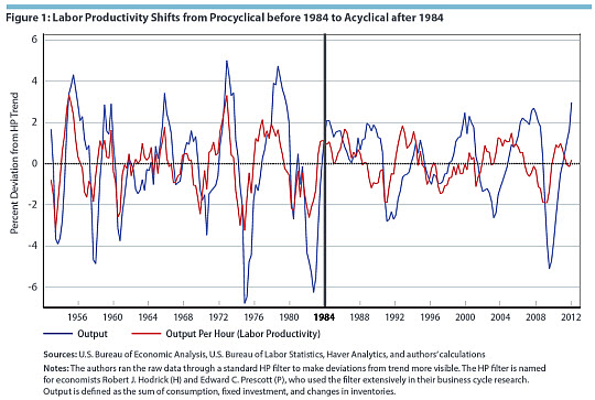
While economists scrambled to explain why output had become less volatile after 1984, they paid considerably less attention to the fact that the comovement of some key economic aggregates had changed as well. Prior to 1984, for example, labor productivity (defined here as output per hour) was strongly procyclical. In other words, it closely followed the ups and downs of business cycles. But after 1984, labor productivity became nearly acyclical. (See Figure 1.) In other words, it no longer moved in concert with the business cycle. At the same time, labor productivity switched from comoving positively with hours worked before 1984 to comoving negatively with hours worked after 1984. (See Table 1.) Both of these changes challenged the notion that the productivity shocks used in the standard RBC model drive business cycles all by themselves. Given that physical capital changes slowly, labor productivity effectively serves as a proxy for productivity shocks as long as it moves in tandem with output. But changes to that comovement and to other patterns of labor productivity in the mid-1980s suggest that other types of shocks likely were playing a larger role than they do in the standard RBC model.

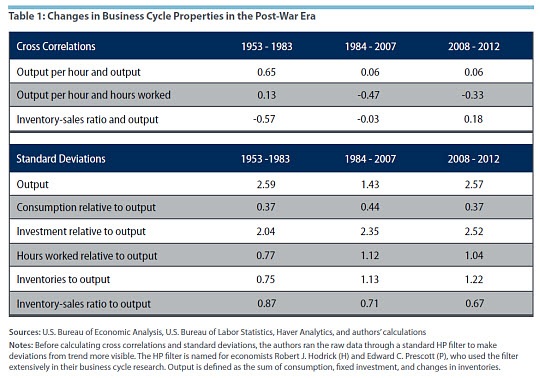
In addition to changes in these comovements, the volatility of hours worked relative to output (expressed in Table 1 as the standard deviation) increased 45 percent – from 0.77 to 1.12 – after 1984, which suggests changes in frictions govern­ing labor markets as firms became more willing to adjust their workforces over the business cycle both on the extensive margin (the number of employees) and the intensive margin (the number of hours the average employee works). Finally, the countercyclicality of the inventory-sales ratio vanished after 1984. At the same time, the volatility of inventories relative to output increased more than 50 percent — from 0.75 to 1.13.

The shifts in relative volatilities and comovement patterns documented in Table 1 persisted through­out the Great Recession, suggesting that this most recent downturn was typical of post-1984 business cycles even though it was on a much larger scale. In other words, even though the Great Recession was significantly deeper than the recessions of 2001 and the early 1990s, the dynamics of the underlying eco­nomic relationships were essentially the same.

Inventories to the Rescue

Three coauthors of this Economic Brief (Lubik, Sarte, and Schwartzman) attempt to explain post-1984 business cycles by extending the neoclassical RBC model presented by University of Rochester economists Robert G. King, Charles I. Plosser, and Sergio T. Rebelo in 1988.⁸ To this basic framework, Lubik, Sarte, and Schwartzman add multiple stages of production, productivity shocks that affect different sectors in different ways, and both permanent and temporary shifts in production possibilities.⁹

At the core of their expanded model are stages of production – a lengthy process that starts with planning and design and progresses through coordination of suppliers, manufacturing of products, distribution to retailers, and ultimately sales to consumers. During the latter stages of this process, inventories of various types sit in factories, warehouses, and stores, waiting for the next step.¹⁰ The model's stage-of-production feature combines detailed production structures from the RBC literature with a mechanism that allows (and, in fact, provides an important incentive for) firms to effectively redirect some of their currently available labor and capital toward the production of goods in the future. This redirection of resources is what gives rise to inventories.¹¹ This extension of the standard RBC model allows researchers to capture an extensive set of changes to production possibilities that might otherwise be assigned to fluctuations in preferences over consumption and leisure in RBC models without inventories.

Analyzing inventory behavior in this way further enables researchers to distinguish variations in the physical return to investment from variations in the discount rate – effectively the interest rate that firms use to assess the present value of future income streams. Variations in the discount rate become distinguishable because they affect inventories as well as fixed investment in similar ways, whereas variations in the return to investment affect fixed investment disproportionately. The discount rate influences how firms allocate resources over time, and these decisions are reflected in levels of inventories. So a substantial increase in fluctuations of inventories relative to output (captured by a less countercyclical inventory/sales ratio) indicates that variations in the discount rate have become key drivers of post-1984 recessions. This conclusion differs substantially from RBC models without inventories that point to changes in the valuation of leisure as key drivers of these recessions. Changes in the valuation of leisure remain important actors in the extended model, but they now share the stage with fluctuations in the discount rate.

The researchers test their results by comparing their estimates of variations in the discount rate to other independent measures of credit-market frictions. They find that the measure that emerges from their model correlates well with a wide array of measures of credit-market frictions, including the lagged spreads between Treasury bonds and Baa-rated bonds, dividend payouts to business owners, and the fraction of U.S. banks that tighten lending standards.

In the spirit of the RBC literature, Lubik, Sarte, and Schwartzman attempt to gauge how well variations in technology alone account for the changing nature of business cycles. They find that the effects of fluctuations in technology are qualitatively in line with various comovement properties and relative volatilities of economic aggregates prior to 1984, but they are unable to account for the bulk of the variation in hours worked after that date and, therefore, changes in the behavior of labor productivity.

The researchers also use their model to see what business cycles would look like if they did not allow any of the multiple fundamental shocks that ultimately drive the economy to have any effect whatsoever on variations in the discount rate. In this scenario, the model fails to produce some of the salient business cycle facts (such as those presented in Table 1) in the period following the Great Moderation. Conversely, when the researchers perform a similar exercise using an RBC model without inventories, they find no role for discount rate fluctuations. It is as if financial shocks and frictions are everywhere except in the macroeconomic data — to pilfer a phrase from Nobel laureate Robert M. Solow.

Either way, the results indicate that more detailed models of business cycles should incorporate some role for financial frictions in order to explain the comovement and relative volatilities of key economic aggregates in post-1984 business cycles.

Back to the Future

Adding a stage-of-production feature to the standard RBC model to incorporate the role of financial frictions harkens back to the complexity of Mitchell's early business cycle research. In 1952, Berkeley economist Robert A. Gordon concluded that "Mitchell was nearer the truth than the recent builders of aggregative models when he insisted on emphasizing the range and complexity of the relations which are relevant to a study of business cycles." In the same article, however, Gordon faulted Mitchell for emphasizing "that there was one, essentially un­changing response mechanism, the delineation of which was to be the main step in explaining the business cycles of the last one hundred years or more."¹²

Thomas A. Lubik is group vice president for micro­economics and research communications, Karl Rhodes is a senior managing editor, Pierre-Daniel G. Sarte is a senior advisor, and Felipe F. Schwartzman is an economist in the Research Department at the Federal Reserve Bank of Richmond.

This article may be photocopied or reprinted in its entirety. Please credit the authors, source, and the Federal Reserve Bank of Richmond and include the italicized statement below.

Views expressed in this article are those of the authors and not necessarily those of the Federal Reserve Bank of Richmond or the Federal Reserve System.