How Data Revisions and Uncertainty Affect Monetary Policy
Economic Brief
January 2026, No. 26-01
Key Takeaways
- Important macroeconomic data are often revised, and initial releases are subject to sometimes large measurement errors.
- The size of the data revisions has declined over time for most key series, but discrepancies between initial and final data for some variables are not random.
- This creates a problem for policymakers, since they need to make decisions in real time while not knowing the true state of the economy.
Most macroeconomic data are subject to frequent and regular revisions. A prime example is quarterly GDP, which is published by the Bureau of Economic Analysis (BEA). Typically, at the end of the first month after the reference period (say, April for first quarter GDP), the BEA releases an advance estimate. A second estimate follows a month later, and a third (labelled "final") estimate is published a few weeks later, almost an entire quarter after the reference period.
But revisions do not stop there. The BEA revises its GDP estimates annually, typically in late September. These annual revisions are designed to refine the higher frequency estimates as more complete data — such as data from the Census Bureau on farm statistics — become available. Annual revisions are not necessarily restricted to the prior year but can sometimes go back several years. Also, the BEA conducts comprehensive revisions every five years to implement methodological changes on how the economy is measured, to update how certain activities are counted and to incorporate new data sources.
Frequent revisions are a function of the frequency of data releases. If GDP were reported only annually, then the BEA would have more time between reports, increasing confidence in measurement and reducing the need for revisions. Moreover, measured GDP includes numerous components that are imputed or not directly calculated. The largest such component is owner-occupied housing, which represents the implicit rent that homeowners pay themselves. Information underlying such imputations often becomes available only with a considerable lag or at lower frequency. Lastly, even if data are measured precisely based on market activity (such as retail sales), the size of the economy and the complexity of data collection make sampling necessary. The timeliness of GDP measurement thus rests on the speediness of the reports.
At the same time, some important series are never revised. The unemployment rate is one notable example: It remains unrevised because it is a survey-based measure and reported as-is, subject to all the concerns that this entails. But by and large, key economic data are constantly revised.
How Big Are the Revisions to Macroeconomic Data?
We now investigate how big the revisions in some key macroeconomic data are. Later, we assess how potentially problematic any mismeasurement — especially for the conduct of monetary policy — could be. We use data from the Philadelphia Fed's Real-Time Data Research Center, which collects vintages of U.S. data releases. We compare the initial release to its final reported value. The difference between these two is our measure for the extent of revisions.
Real GDP
Figure 1 shows the revisions to annualized quarterly GDP growth in terms of percentage points since the 1960s, measured as the difference between the initial and final releases. The full sample shows two distinct periods — namely before and after 1983 — where a statistically significant break in the revision series occurred. This coincides with what is often referred to as the Great Moderation (that is, a decline in macroeconomic volatility after 1983).

The mean of the revisions is a statistically significant 0.45 percentage points (pp), as seen in Table 1. That is, on average, annualized quarterly GDP growth is initially underreported by about half a percentage point. Ideally, this measurement error would be zero. Instead, these revisions suggest that the economy is typically stronger than it initially appears. For example, the initial estimate of second quarter GDP in 2025 came in at 3.0 percent and was revised upward in the final estimate to 3.8 percent.
| Period | Mean | Median | Standard Deviation |
|---|---|---|---|
| Full Sample | 0.45* | 0.34 | 1.97 |
| 1965 to 1983 1983 to 2025 | 0.69* 0.35* | 0.47 0.32 | 2.74 1.55 |
| Note: * denotes p < 0.05. Source: Bureau of Economic Analysis and authors' calculations. | |||
The standard deviation for the full sample is 1.97, which is four times as large as the mean and indicates a considerable degree of variation. This suggests that, as a rule of thumb, two-thirds of all revisions lie in a range of -1.52 percent to 2.42 percent. Naturally, this includes some sizeable revisions during periods of economic turmoil in the 1970s, the financial crisis in 2007-09 and the pandemic in 2020.
The patterns in the revisions seem to have changed after 1983, when the standard deviation declined to 1.55 from a pre-1983 value of 2.74. Furthermore, the mean decreased to 0.35pp after 1983 from a value of 0.69pp before. In other words, the government statisticians erred a lot in both directions (especially in the 1970s), more often underestimating than overestimating. After 1983, however, they became more accurate, with initial estimates exhibiting less downward bias.
One important consideration is whether the revision mean is the right statistic to examine when trying to think through the apparent bias in initial estimates. An alternative measure is the median, which is the value at which half of the revisions are above or below. Importantly, the median is not pushed around by outliers such as during periods of turmoil. In the full sample, the median of 0.34pp is below the mean, but still positive. The higher pre-1983 median (0.47pp versus 0.32pp for post-1983) indicates that downward bias was relatively ubiquitous before 1983, not just due to the influence of outliers.
PCE Inflation
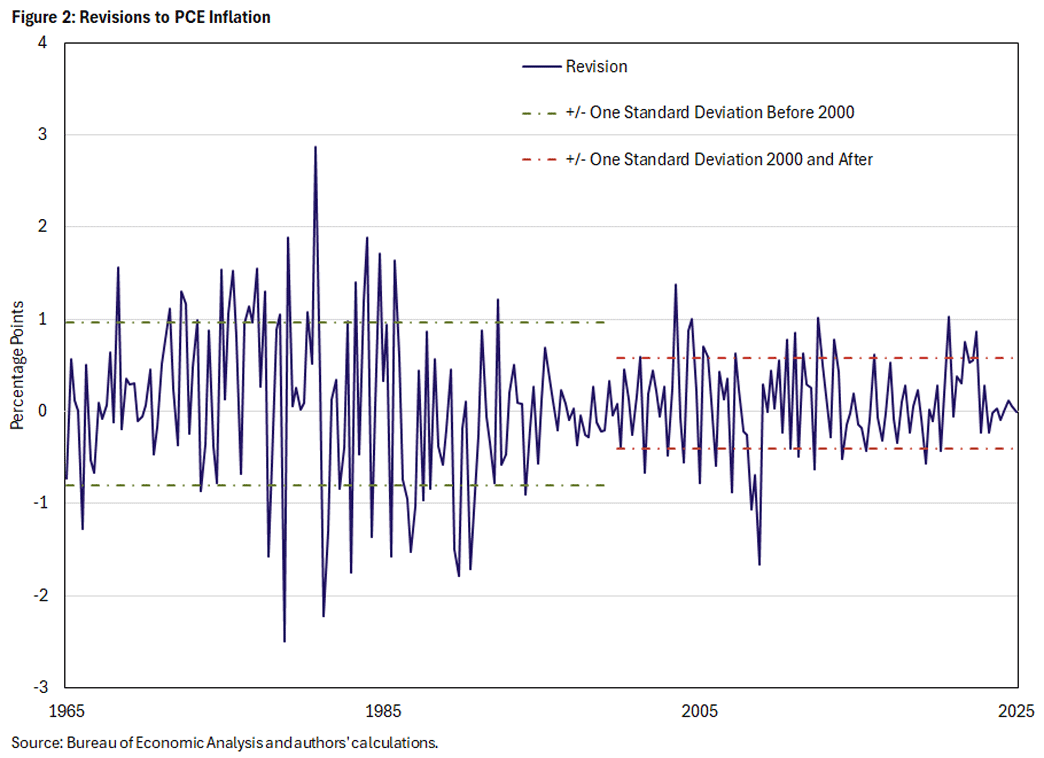
Figure 2 looks at revisions of the Federal Reserve's preferred inflation measure: the PCE price index. We report annualized quarter-over-quarter numbers. The figure shows a break in the revision series in 2000, when the series became visibly and notably less volatile. We do not find a break in 1983 as for GDP but report the corresponding numbers for reference purposes in Table 2.
| Period | Mean | Median | Standard Deviation |
|---|---|---|---|
| Full Sample | 0.08 | 0.08 | 0.74 |
| 1965 to 2000 2000 to 2025 | 0.07 0.09 | 0.08 0.09 | 0.89 0.49 |
| 1965 to 1983 1983 to 2000 | 0.22* -0.09 | 0.25 -0.08 | 0.92 0.83 |
| Note: * denotes p < 0.05. Source: Bureau of Economic Analysis and authors' calculations. | |||
The mean and median of the revisions are essentially identical between the pre-2000, post-2000 and the full sample periods, suggesting no outliers. Similarly, the means are close to zero and not significant, so the revisions in PCE inflation closely resemble classical measurement error in an econometric sense without much (if any) bias. One exception is the period before 1983 with a significant mean revision of 0.22pp, suggesting a slight understating of inflation driven by the 1970s.
Payroll Employment
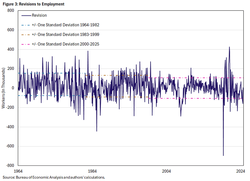
Finally, we look at revisions to payroll employment in Figure 3 and the respective statistics in Table 3. Although employment revisions attract a lot of attention — a case in point being the benchmark revision in July 2025, which revised down total employment by 500,000 over the last year — the revision series looks remarkably well behaved. Sample mean and medians do not differ much, and the revision mean is significant but close to zero, especially after 2000.
| Period | Mean | Median | Standard Deviation |
|---|---|---|---|
| Full Sample | 17.4* | 17.5 | 111.6 |
| 1964 to 1983 1983 to 2000 2000 to 2025 | 35.7* 22.8* 0.8 | 39.5 21.5 1.0 | 116.3 111.6 106.0 |
| Note: * denotes p < 0.05. Source: Bureau of Economic Analysis and authors' calculations. | |||
Patterns and Recession Indicators
We also perform some simple analyses to see whether there are systematic patterns in the revisions and whether they allow us to make inferences about recessions. With respect to the former, GDP and inflation measures show negative first-order correlation that is not statistically significant. That is, large revisions tend to be followed by considerably smaller revisions in the opposite direction. This suggests that revisions in these variables are measurement error (even when biased) and that there is some degree of mean-reversion. The exception is employment, which is significantly positively serially correlated. This means that revisions in the same direction come in clusters and thus have a predictable component. Finally, we consider revisions in the four-quarter run-up to NBER recession dates, but we do not find much of a pattern.
Overall, we find that data revisions — the discrepancy between initial and final releases — can be substantial: They tend to differ from zero on average but do not show systematic biases, perhaps with the exception of GDP growth. Nevertheless, the possibility of such revisions creates a problem for policymakers as they need to conduct policy based on the data available, not necessarily knowing the final readings. This is often called real-time policymaking and creates its own set of issues.
How To Think About Real-Time Policymaking When Data Are Mismeasured
From an economic theory perspective, we can think of revisions as a specific form of data uncertainty. Even if economic actors know and understand the model of the economy, some important variables (such as the natural real rate of interest r*) may not be observable, while the data for other variables may be subject to revisions. We can thus think of the initial observable data release as subject to measurement error. The economic literature has studied the implications for monetary policy extensively.
Perhaps the best-known application of monetary policy under uncertainty is the Brainard principle.1 If a policymaker is uncertain about the effects of their actions — for instance, how business lending responds to interest rate changes — the policy prescription is to respond more cautiously and adjust policy less aggressively than in the absence of uncertainty. This prescription is called attenuation. It stems from the observation that the central bank must figure out what the true relationships characterizing the economy are. If policymakers acted as if they knew, they would run the risk of overshooting, in turn potentially exacerbating volatility. A loss-minimizing policymaker therefore proceeds more cautiously when uncertain. More recently, however, this aspect has come under scrutiny theoretically and empirically.
The Best Laid Plans of Mice and Men ...
In my (Thomas') 2016 paper "Indeterminacy and Learning: An Analysis of Monetary Policy in the Great Inflation" — co-authored with Christian Matthes — the monetary policymaker does not know the full structure of the economy but understands that GDP and inflation evolve as functions of their lagged values. In this environment, the central bank can try to understand the dynamics in the economy by estimating a vector autoregression (VAR) model, which describes how key aggregate variables evolve over time. In fact, by doing this for a sufficiently long time span, the central bank will eventually be able to learn the true dynamic structure of the economy. There will be errors for shorter periods, and these errors are potentially compounded if the data used for estimating the VAR model contains measurement error, as it typically does in the case of initial data releases.
In this framework, the central bank solves an optimal policy problem where it sets the nominal rate to minimize the variation in GDP and inflation, given the current estimates of the economic dynamics. If there is measurement error in the data, the implied optimal policy choice is likely biased. For instance, if the advance estimate of GDP growth comes in lower than its final value, the central bank may optimally choose to be more accommodative than it should. It may therefore inadvertently violate the Taylor principle, which posits that policy should be such that it raises the real rate of interest in face of a stronger economy or a softer inflation outlook.
This insight is central to the argument in my (Thomas') 2016 article — co-authored with Matthes and Tim Sablik — that this is exactly what happened in the 1970s. While the Fed under Arthur Burns has been blamed for causing the Great Inflation by not adopting an aggressive-enough anti-inflationary stance, the presence of significant data revisions (seen in Figures 1 and 2) suggest that the Fed did its best given the circumstances. Luckily, the volatility, size and range of data revisions have broadly declined since then, so this issue is probably less of a concern today.
The Perils of Knowing Just Not Enough
My (Thomas') 2023 paper "Indeterminacy and Imperfect Information" — co-authored with Matthes and Elmar Mertens — uncovers another (perhaps more disturbing) theoretical channel of how data revisions can affect outcomes. The article assumes that policymakers operate under rational expectations but with limited information. Specifically, a subset of economic actors has access to less information than the fully informed ones. Information limitations are such that some policy-relevant variables are not observed, and observed variables are subject to measurement error. This constitutes a small but critical deviation from a full information setting where all agents in the model (households, firms and policymakers) know the structure of the model (how the economy works, what the shocks are, and how all other agents in the economy behave) and form expectations about the future rationally.
As an example, these assumptions describe an economy with a central bank that follows a Taylor rule but does not know r*. Consequently, policymakers operate in a real-time environment, where the first data release is subject to potential future revisions. How can policy be conducted when the central bank does not know the values of the right-hand side variables in the rule? Well, the policymaker must form expectations about the unknown variables. As it turns out, the central bank's optimal projection or expectation is an updating equation that takes a signal — for instance, a new data release or information that allows some inference about unobservable r* — weighs it against the known existing information and forms an estimate of the variable of interest. The relative weight on the new versus existing information depends on the historical average information content of the new data, including on whether historically there was a lot of noise or not. Crucially, this signal extraction process — which seems a priori a perfectly sensible thing to do — risks creating self-fulling expectations and sub-optimal outcomes.
Self-Fulfilling Expectations in a Real-Time Environment
Suppose consumers believe that incomes or income growth (because of, say, AI-driven productivity gains) are higher than the data indicate. This could trigger additional consumption demand beyond what is consistent with the fundamentals. This raises inflation in a standard monetary policy model, and the central bank is bound to react.
If policy follows the Taylor principle, the central bank will raise the nominal rate more than proportional to the notional increase in inflation, thus raising the real rate, which in turn reduces the additional consumption demand and stamps out incipient inflation. If it is understood that the policymaker would react in this way, such beliefs would not have taken hold in the first place.
On the other hand, if policy does not follow the Taylor principle, then the central bank's response would lower the real rate, providing a consumption stimulus and thus validating the initial beliefs. In this scenario, the economy exhibits self-fulfilling fluctuations because of the policymaker's (non)actions.
In an economy with measurement errors in the data, the same mechanism is at play, but with an additional twist. Suppose economic agents believe that inflation is lower than it actually is. The central bank then uses its information-updating equation to adjust its assessment of current inflation. Since this is weighed between the current data-based information and the belief-driven new signal, some weight will be placed on the latter. The central bank thus lowers its assessment of "true" inflation and lowers the policy rate. This generically lowers the real rate: With policy now less restrictive or perhaps even expansionary, inflation rises. Even if the Taylor principle applies, the real rate falls and thus validates the belief in a lower inflation rate.
The core of the self-validating belief mechanism in this scenario is that the central bank is assumed to follow a projection-based rule. Because of the attenuation principle embedded in the updating equation, the presumptive policy rule is turned into an effective policy rule, which softens (attenuates) the Taylor principle so that the actual central bank actions resemble passive monetary policy. This can simply be avoided by not following a projection-based rule (that is, by not trying to "see through" the real-time data and instead respond to the data as they are).
Summary
There is much uncertainty about data uncertainty. For one, there is some evidence that measurement error in key macroeconomic data — specifically the difference between initial and final releases — is not purely measurement error, but that at the very least its magnitude has decreased over time. Nevertheless, the difficult problem for policymakers remains how to conduct policy in a real-time environment without full knowledge of the state of the world. Recent research has shown that, despite their best intentions, policymakers can get it wrong and pursue unwittingly suboptimal policies.
Thomas Lubik is a senior advisor, and Jacob Titcomb is a research associate, both in the Research Department at the Federal Reserve Bank of Richmond.
1
Established in the 1967 paper "Uncertainty and the Effectiveness of Policy" by William Brainard.
To cite this Economic Brief, please use the following format: Lubik, Thomas A.; and Titcomb, Jacob. (January 2026) "Data Revisions and Uncertainty: How They Affect Policy." Federal Reserve Bank of Richmond Economic Brief, No. 26-01.
This article may be photocopied or reprinted in its entirety. Please credit the authors, source, and the Federal Reserve Bank of Richmond and include the italicized statement below.
Views expressed in this article are those of the authors and not necessarily those of the Federal Reserve Bank of Richmond or the Federal Reserve System.
Subscribe to Economic Brief
Receive a notification when Economic Brief is posted online.
Contact Us