The Natural Beveridge Curve

The Beveridge curve is a staple for analyzing the state of the labor market. It depicts the relationship between the unemployment rate and the vacancy rate (that is, the number of open positions or available jobs relative to the set of potential job seekers). It is typically depicted as a scatterplot of the two variables, from which a clear negative or downward-sloping relationship emerges, as shown in Figure 1.

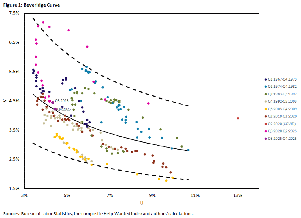
In the figure, we color-coded quarterly vacancy-unemployment combinations such that they correspond to fluctuations in the unemployment rate, from peak to trough to subsequent peak. While the graph shows a downward-sloping relationship over the full sample, individual cycles also show Beveridge curve behavior. For instance, the 1974-82 or 2003-09 groupings show downward slopes within just their respective timeframes.

We also estimated a regression on the full sample (the solid line) and the associated standard error (the dashed lines). Since the uncertainty region essentially covers all data points, we cannot rule out the existence of a single underlying relationship, despite the noticeable shifts in individual Beveridge curves.

However, Figure 1 still suggests that individual Beveridge curves can be identified and that the position of each is subject to economic forces. Intuitively, the Beveridge curve reflects the state of the business cycle: When times are good, businesses want to post open positions and hire, and consequently, the unemployment rate is low. When times are bad, the opposite reasoning applies.

Over the course of the cycle, the labor market moves along the curve. But what is also clearly noticeable from the figure is that the relationship can shift sideways, either outwards or inwards. That is, at the conclusion of a cycle, the location of the Beveridge curve is different as it tends not to return to where it started.¹ These shifts tend to be larger in the wake of longer and deeper recessions or expansions.

Analysis of the Beveridge curve is thus likely to conflate cyclical and structural changes in the labor market, since any point in the scatterplot is determined by the state of the business cycle — whether current labor demand is strong or weak — and by structural forces that affect the functioning labor market. Analysis of the Beveridge curve as it relates to the state of the economy requires disentangling these influences.

This insight is important for policymaker responses to the labor market. Monetary policy actions can affect businesses' willingness to hire and thus help stabilize the economy along the Beveridge curve. In contrast, such measures are unlikely to affect structural changes in the labor market such as improvements in labor market matching through online job postings.

In this article, we attempt to disentangle the two components in the raw Beveridge curve relationship by deriving the natural Beveridge curve. We do so by estimating equilibrium or long-run levels of unemployment and vacancies, which we then combine in a scatterplot. This also allows us to introduce the idea of a Beveridge curve gap as a measure for the cyclical component in the labor market.

Estimating the Natural Rates of Unemployment and Vacancies

We estimate the natural rates following the methodology developed by Christian Matthes and one of us (Thomas).² It is based on a time-varying parameter vector autoregressive model (TVP-VAR), which is a flexible framework for analyzing the dynamics of macroeconomic time series, especially in the presence of structural change and periods of varying economic volatility. Natural rates are computed as the medium-term forecasts from the estimated TVP-VAR, based on the underlying ideas that temporary disturbances will fade away over time and that the economy returns to its normal or natural level.

We use quarterly data for the unemployment and vacancy rates from the first quarter of 1959 to the fourth quarter of 2025. We compute the vacancy rate from the number of job openings remaining unfilled on the last day of the month as measured by the Bureau of Labor Statistics' Job Openings and Labor Turnover Survey (JOLTS) from 2001 to the end of the sample. This series is spliced together with the composite Help-Wanted Index created by economist Regis Barnichon available from the beginning of the sample.³ The vacancy rate is calculated in the same way as the openings rate released by JOLTS, namely the total number of vacancies divided by the sum of total employment and total vacancies. Figure 2 shows the vacancy rate and its estimated natural rate V*.

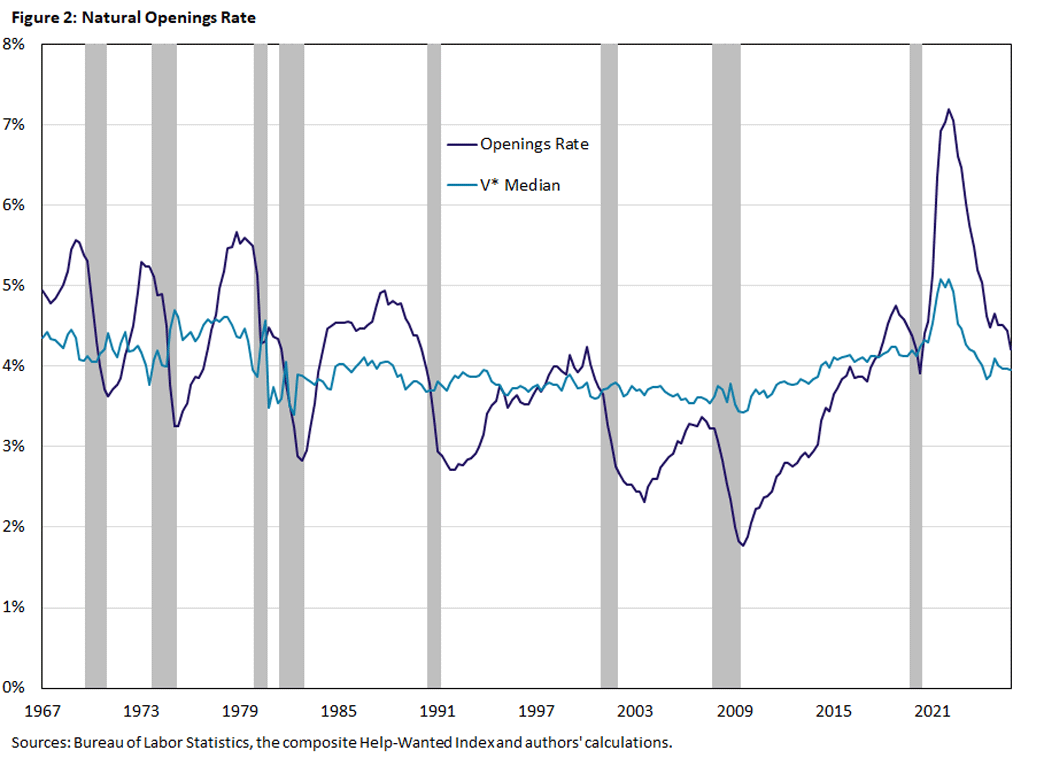
The vacancy rate exhibits a notable decline from 4.5 percent at the beginning of the sample to a trough of 1.8 percent in 2010. The ups and downs of measured job openings coincide with expansions and downturns (that is, the procyclicality of vacancy postings). From 2010 on, vacancies appear to be on a secular rise, from the trough at 1.8 percent to around 4.2 percent, abstracting from the spike during the pandemic recovery.

At the same time, the natural vacancy rate is remarkably stable from the early 1980s until 2010, when it started rising by a full percentage point. Its maximum level over the sample period is 5.1 percent in the first quarter of 2022, but it has come down to its current level of 4.0 percent.

As a first pass (and intuitively), we can think of vacancies as reflecting the labor demand side of the economy. If firms want to hire, they need open positions (vacancies) first. Labor demand shifts with the state of the economy, as can be seen in Figure 2. But what underpins this dynamic is what may be called structural labor demand, which is captured by V*.

The determinants of V* are generally the cost of hiring (the more costly hiring is, the lower is V*) and the ease with which open positions can be filled. The latter includes the overall efficiency of how job seekers and job openings are combined to yield employment ("match efficiency") and the responsiveness of matches to changes in job seekers ("match elasticity").

The rise in V* thus potentially signals structural change in the labor market: Over the course of the sample period, it has become easier to post vacancies on account of online job postings and recruiting, while at the same time the efficiency of labor matching seems to have decreased. That is, to hire additional workers, employers need to recruit more and more actively.

Our estimate of V* also indicates that a substantial fraction of the rise in vacancies after the pandemic was structural. At the same time, structural increases in vacancy posting already started in 2010, where it is tempting to associate this with the growth of online job search.

Figure 3 shows the corresponding estimates for the unemployment rate and U*.

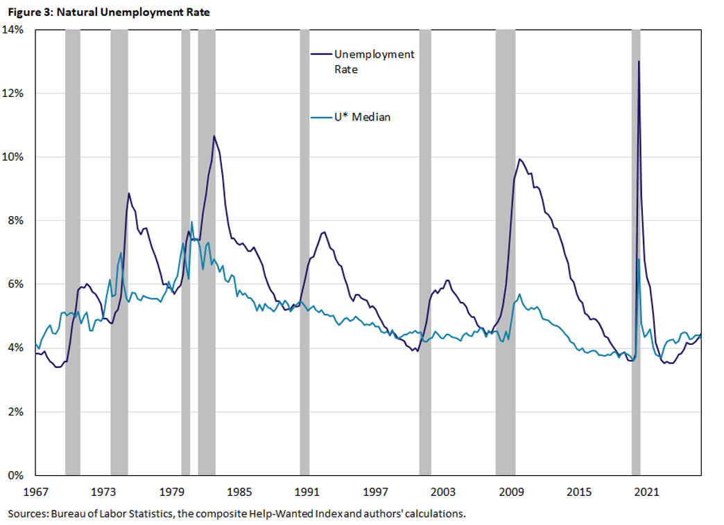
In contrast to the natural vacancy rate, U* shows more variation as it generally follows the ups and downs of measured unemployment. We can observe some differences before and after the 1980s. In the 1970s, the natural rate of unemployment was on the rise, increasing with every recession. This pattern changed with the Volcker disinflation of the early 1980s after reaching a level of close to 8 percent. U* reached a trough of 4 percent by the late 1990s before hovering around 4.2 percent to 4.6 percent from 2000 to 2008. Notably, the two recessions in 1990-91 and 2001 did not appear to affect the natural rate.

This changed with the Great Recession of 2007-09, which drove U* up by a full percentage point. The subsequent recovery, on the other hand, led to a decline in U* to its lowest level over the sample (3.6 percent). Similarly, the pandemic recession of 2020 led to a spike in U*, which now stands at 4.3 percent, the same level as measured unemployment. This pattern suggests that changes in U* are due to longer-term factors such as demographic changes in the labor force or are driven by extraordinary recessions.⁴

The Natural Beveridge Curve

Figure 4 combines the estimates of U* and V* as a scatterplot to show the natural Beveridge curve. As in Figure 1, different colors indicate specific periods that we align with fluctuations in the unemployment rate.

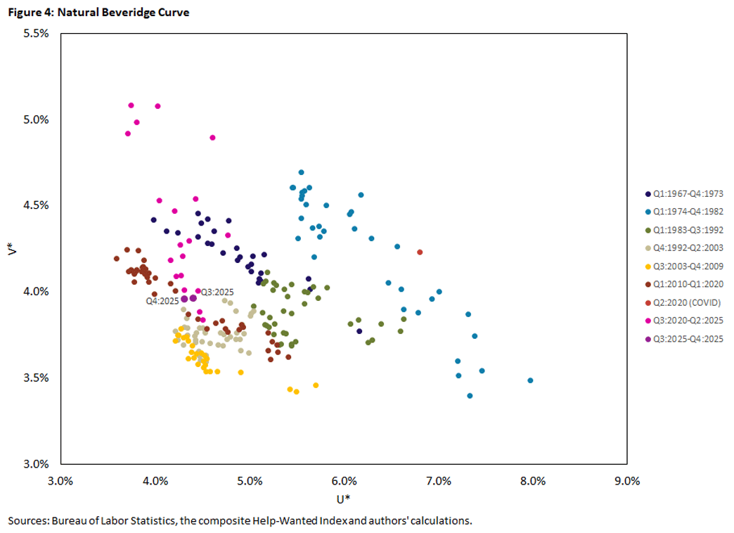
Naturally, there is much less variability in the natural Beveridge curve than in the one based on measured data in Figure 1, as can be gleaned from figures 2 and 3. Abstracting from the Great Inflation period of 1973-85, both U* and V* move in a 1.5-percentage-point range. Visually, the cycle-specific natural curves line up with those identified in the underlying data in Figure 1, as can be expected when the "trend"⁵ in the unemployment and vacancy rates is a smoother version of the data.

What does the natural Beveridge curve represent? Just like the natural rates of unemployment and vacancies, it captures a state of the economy where the labor market is at rest in the sense that it is no longer buffeted by temporary disturbances. It can still move around, but these movements are by definition due to a long-run structural change, such as the changes in how well the matching process between job seekers and open positions works. The gap between the Beveridge curve and its estimated natural counterpart can therefore give an assessment of the shorter-term pressures on the labor market that policymakers can hope to influence.

The Beveridge Gap

Figure 5 shows an alternative representation of the Beveridge curve relationship. It depicts the difference between measured labor market tightness — namely, the ratio of vacancies to unemployment — and its natural level. Tightness is a central concept in the search and matching approach to the labor market. We call a labor market "tight" when the number of vacancies is high relative to the number of potential job seekers, as firms would find it difficult to hire. In contrast, having few open positions when many workers are unemployed implies a looser labor market, as it is comparatively easy to fill positions. In a sense, the V/U series represents the Beveridge curve compressed from a scatterplot into a time series. This illustrates the gap between actual and natural values in an arguably cleaner manner.

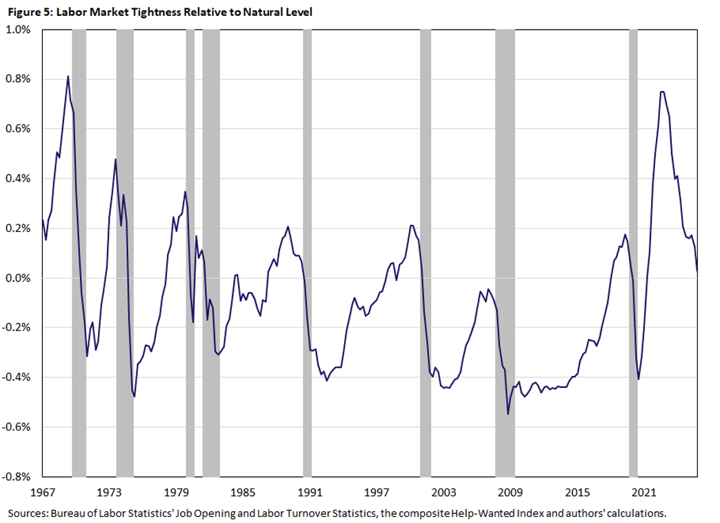
The tightness gap can be interpreted as the cyclical movements in the Beveridge curve variables net of the structural changes encapsulated in the respective natural rates. As such, the graph yields some interesting observations.

First, the labor market is rarely in its long-run equilibrium captured by the natural Beveridge curve as it crosses zero generally only once over the course of an expansion.

Second, the gap is on average negative, even when abstracting from the deep recession in the financial crisis. That is, tightness is generally below its natural level, which indicates a deficiency of vacancies and/or a surplus of job seekers. Arguably, this suggests a general lack of labor demand over the course of an economic cycle.

Third, we see that the tightness gap generally rises steadily during an expansion, which is perhaps not surprising. Driving this is the rise in vacancy rate and the decline in unemployment following a recession, as observed in figures 2 and 3.

Fourth, the pattern in the Beveridge curve during the pandemic and in the following years — which looks like an extreme outlier in Figure 1 — is not as dramatic in Figure 5. The tightness gap in the 2020s barely reaches its peak of the 1970s. This suggests that much of the run-up in vacancies during this time was structural, as reflected in the natural rate of vacancies. This finding is in line with the argument in a 2024 paper that the decline in the vacancy rate following its peak after the pandemic has no inflationary impact and does not signal weakness in the labor market, as V and V* were coming down at similar rates.⁶

Fifth, tightness shows a downward trend for most of the sample period, though recently it appears to stabilize or perhaps even reverse. This indicates that the actual strength of the hiring process was falling behind its potential (or natural) level over time, perhaps consistent with the notion of jobless recoveries evident already in the recession in the early 1990s and later on. This process seems to have gone in reverse after the Great Recession where both actual and potential hiring improved, the former more so than the latter. This might also explain why the actual Beveridge curve has a much more noticeable slope, while the natural Beveridge curve is quite flat.

Summary

We have introduced the notion of the natural Beveridge curve, which describes and summarizes the state of the labor market in the longer run by abstracting from transitory movements. As such, the Beveridge gap between the actual and potential data shows that there is room for stabilizing vacancy postings since the natural vacancy rate has historically been quite steady. Structural factors have a bigger effect on the natural unemployment rate. Understanding the natural Beveridge curve thus gives policymakers a better handle on the efficacy of labor market stabilization policy.

Katherine Anderson is a research associate, and Thomas Lubik is a senior advisor, both in the Research Department at the Federal Reserve Bank of Richmond.

To cite this Economic Brief, please use the following format: Anderson, Katherine; and Lubik, Thomas A. (May 2026) "The Natural Beveridge Curve." Federal Reserve Bank of Richmond Economic Brief, No. 26-17.

This article may be photocopied or reprinted in its entirety. Please credit the authors, source, and the Federal Reserve Bank of Richmond and include the italicized statement below.

Views expressed in this article are those of the authors and not necessarily those of the Federal Reserve Bank of Richmond or the Federal Reserve System.