How Do Real Exchange Rates Vary in Hard and Soft Sovereign Defaults?
Sovereign defaults differ tremendously in creditor losses. Existing research has established that hard defaults (large creditor loss defaults) are associated with worse outcomes for GDP per capita than soft defaults. In this article, we document that hard defaults also feature worse real exchange rate depreciations.
Sovereign default occurs regularly in emerging countries (such as Malaysia recently) and occasionally in developed ones (such as Russia in April and Greece a decade ago). Yet, defaults differ tremendously in their intensity with commensurate consequences for both lenders and sovereigns. As shown in the 2017 paper "The Output Costs of Hard and Soft Sovereign Default" by Christoph Trebesch and Michael Zabel, these differences are systematic:1
- Hard defaults — defined as defaults with large losses for lenders — are characterized by large, persistent declines in GDP per capita.
- Soft defaults — those with small losses — are associated with a small, temporary dip.
In this article, we report that real exchange rates (RERs) also vary systematically depending on default intensity.
Real Exchange Rates vs. Nominal Exchange Rates
Both RERs and nominal exchange rates (NERs) are measures of purchasing power. In simple terms, the more familiar NER answers the question "How much foreign currency does it take to buy one dollar?" The RER instead answers the question "How many foreign good baskets does it take to buy one unit of the U.S. basket?"2
Stated this way, RER depreciations — reductions in the purchasing power of foreign goods — are increases in the RER. As found in our paper "A Quantitative Theory of Hard and Soft Sovereign Defaults," RER depreciations are larger in hard defaults than soft defaults.
Measuring Sovereign Defaults and Real Exchange Rates
For our analysis, we build off the dataset constructed by Trebesch and Zabel. Specifically, we obtain from the paper data covering real GDP per capita, default status and losses. The paper focuses only on the debt restructurings that allowed countries to cure default without re-entering a new default episode within four years. Thus, there is only one final loss reported per default episode. The full sample spans the period 1980 through 2009 and includes 33 default episodes from 25 developing and emerging market economies. (Several countries have more than one default.)
We supplement this database with various measures of RERs constructed using data obtained from the World Bank and the Penn World Table (PWT). As previously mentioned, the RER is the quantity of baskets that can be bought in country A given one basket in country B.
Suppose the price level in A is P, the price level in B is P*, and the NER is E (which is the amount of currency in A per unit of country B currency). Then, a basket in country B can be converted to P units of currency, which can be exchanged for PE units of country A's currency and then buy EP*/P units of country A's basket. Hence, the real exchange rate is RER = EP*/P. (Some authors use the opposite convention for exchange rates, so their RER is the inverse of this one.)
In our convention, an RER depreciation is an increase in the RER, which is a reduction in the purchasing power of country A. For our purposes, country A will differ depending on the sample, and country B will always be the U.S. Because most external debt in emerging markets is priced in U.S. dollars, this is the relevant RER when it comes to issues related to debt, default and losses.
For this analysis, we will use an RER measure derived from reported price levels for output-side real GDP in the PWT. Through relatively straightforward algebraic manipulations, we obtain our measure of the RER. Theoretically, the PWT strives to measure exactly what we are after, which is holding the entire basket of goods production fixed and measuring the relative cost in two countries. While some in the literature have used the PWT for RER measures, price levels are more commonly obtained using either the CPI, core CPI or the GDP deflator.3
For comparison, we also compute RER using price levels and NERs sourced from the World Bank. Our RER PWT is highly correlated with measures of the RER computed using these alternative measures of a country's price level.4 In addition to being very highly correlated with standard measures of the RER, our RER PWT has the advantage of having broad coverage of the countries and time periods in our sample.
We classify defaults as hard or soft depending on whether the realized losses were above (hard) or below (soft) the median size of losses. With these classifications, we test whether hard defaults are "worse" than soft defaults. That is, we investigate whether, on average, hard defaults correspond with larger contractions in real GDP per capita, greater RER depreciations and longer default durations compared to soft defaults.
Effects of Hard Defaults vs. Soft Defaults
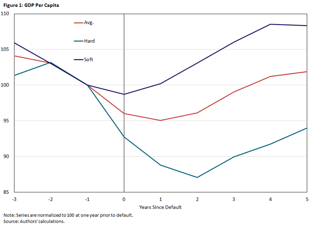
The results of our investigation are summarized in the figures below. In Figure 1, we reproduce the analysis conducted by Trebesch and Zabel using our classification of hard and soft defaults based on loss size.
Although their paper uses a coerciveness index (measure of government's payment and negotiation behavior towards creditors) to classify defaults, it shows that loss size and coerciveness have a strong, positive correlation (approximately 0.7) and suggests that coercive actions during default are a strong predictor of realized losses. For each default episode, the graphed series is real GDP per capita relative to the period before default averaged across either all defaults (the red line), hard defaults (the blue line) or soft defaults (the purple line).
Consistent with Trebesch and Zabel's paper, we find that hard defaults are associated with deeper, more sustained declines in real GDP per capita compared to soft defaults. Whereas soft defaults are associated with relatively small declines in output with the onset of the default that quickly recover to pre-default levels, hard defaults are associated with large declines in output that remain low through the end of our default observation window.
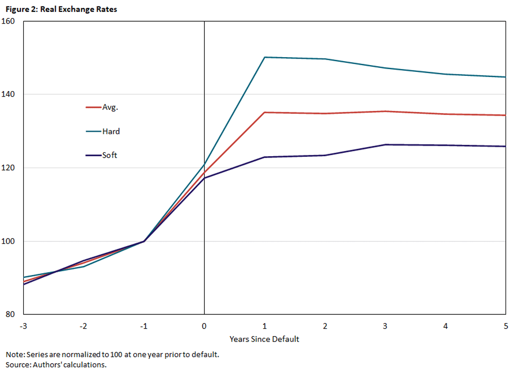
In Figure 2, we do this same exercise using our RER measure.
Here we see hard and soft defaults initially have similar depreciations in the RER with the onset of default. However, in the year following the start of default, the RER in countries experiencing hard defaults continues to increase substantially before leveling off at a rate that is about 50 percent higher than the pre-default RER in the period just prior to default. For soft defaults, the RER begins to level off at a rate about 25 percent higher than the rate just prior to default shortly after the onset of default. While the differences diminish over time, even five years after default, there is still a 20 percent gap.
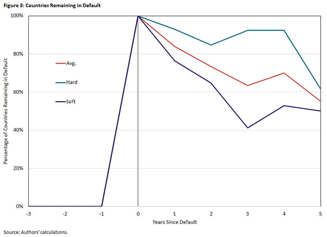
Because default appears to be associated with depreciation, the duration of default episodes may be an important driver of RER. In Figure 3, we plot the proportion of countries still in default five years after default started.
While soft defaults end relatively quickly (with only 40 percent still in default after three years), hard defaults take longer to resolve (with around 90 percent in default after three years).
We also examined the statistical significance of whether hard defaults are worse than soft defaults. In general, our results for real GDP per capita and RER PWT are statistically significant at the 10 percent level. This suggests hard defaults do indeed experience smaller output and greater depreciation than soft defaults. The results for default duration also confirm hard defaults last longer than soft defaults, which — given that RERs depreciate in default — may help explain part of the RER gap in hard and soft defaults.
Conclusion
In this article, we've established that hard defaults are associated not only with larger declines in GDP per capita (as the previous literature did) but also with greater RER depreciations. Additionally, we have shown default duration is longer in hard defaults than soft defaults, which may help explain why these differences in income and RERs persist.
This article has only shown correlation between default intensity and adverse outcomes. Does default intensity cause these outcomes? This is a common view, and Trebesch and Zabel argue for it empirically. However, it also possible for the reverse to be true: Worse outcomes for GDP and the RER may cause default intensity. In our (Grey and Pablo's) ongoing research, this hypothesis is investigated and found to be the main channel linking default intensity and outcomes.
Brandon Fuller was a research associate and Grey Gordon is a senior economist in the Research Department at the Federal Reserve Bank of Richmond. Pablo A. Guerron-Quintana is an economics professor at Boston College.
Trebesch and Zabel use a measure of negotiation coerciveness as their primary definition of default, but they argue their results are robust to defining default intensity using creditor losses.
A "basket" is an important concept in macroeconomics. In this case, a basket is a bundle of goods in amounts equal to that typically consumed. For example, if a "typical" U.S. consumer spends $1,000 on rent for a two-bedroom apartment, $500 on bread at $5 per loaf and $500 on a Ford Escape each month, then the basket would be a two-bedroom apartment, 100 loaves and one Ford Escape. A measure of inflation is how much the price of that basket goes up over time. So, if the price of rent rose 20 percent with the other prices constant, the total cost of the bundle would go from $2,000 ($1,000 + 100*$5 + $500) to $2,200 ($1,200 + 100*$5 + $500), which would be an inflation rate of 10 percent. In reality, baskets are extremely complicated, and inflation measures are corrected for a number of issues. However, the main idea still applies.
An advantage of these is frequency, with CPI and core CPI available monthly, the GDP deflator often available quarterly, but the PWT measure available only annually. Since our other data are annual, there's no loss in sample size from using the PWT.
Robust regressions of these RERs on the RER PWT showed that a 1 percent increase in RER PWT is associated with upwards of an 0.8 percent increase in the standard RER measures (closer to 0.9 percent increase for GDP deflator-based and core CPI-based measures). These regressions also produced R2 measures upwards of 0.8. The CPI and core CPI measures are quite noisy with a number of large outliers in the data, which is why we used robust regressions (which reweight observations to reduce the effects of outliers) for these comparisons.
To cite this Economic Brief, please use the following format: Fuller, Brandon; Gordon, Grey; and Guerron-Quintana, Pablo A. (October 2022) "How Does Default Intensity Affect Real Exchange Rate Depreciations?" Federal Reserve Bank of Richmond Economic Brief, No. 22-40.
This article may be photocopied or reprinted in its entirety. Please credit the authors, source, and the Federal Reserve Bank of Richmond and include the italicized statement below.
Views expressed in this article are those of the authors and not necessarily those of the Federal Reserve Bank of Richmond or the Federal Reserve System.
Receive a notification when Economic Brief is posted online.


