How Concentrated Is the Distribution of Banks' Reserve Balances?

By Russell Wong

Economic Brief

May 2025, No. 25-18

Key Takeaways

We introduce a new concentration measure of banks’ holding of reserve balances: the asset-weighted Gini coefficient, which controls for the differences among banks in size.
In a departure from the traditional measure, the asset-weighted Gini coefficient finds that reserve balances have been more evenly distributed since the 2008 crisis.
The asset-weighted Gini coefficient suggests that ignoring the fact that U.S. banks are vastly different in size would artificially inflate the concentration.

Reserve balances play a critical role in the banking system. Prior to 2020, they satisfied reserve requirements, and they now also serve as the primary payment instrument for settling transactions and client orders via the Fedwire system. Maintaining adequate reserve balances allows banks to meet withdrawal demands and instills depositor confidence, reducing the risk of bank runs. Empirical studies have demonstrated that banks' holding of reserve balances affects the provision of bank credit to firms and households, although the relationship depends on types of credit and methods of reserves being injected into the banking system.¹

Since the Federal Reserve gained the authority to pay interest on reserves in 2008, reserve balances have also become a popular investment for banks. The share of U.S. domestic banks' assets held in reserve balances has increased significantly, rising from less than 1 percent in the first quarter of 2001 to slightly below 6 percent in the third quarter of 2024.

However, despite their importance, reserve balances are not equally distributed across banks. Concerns have been raised about the concentration of reserve balances among a few large banks, particularly following rounds of quantitative easing (three addressing the 2008 financial crisis and one addressing the COVID-19 pandemic). These programs injected substantial reserve balances into the banking system to finance the Fed's purchase of government securities, potentially amplifying concentration concerns.

In response to these issues, we introduce a new measure of reserve balance concentration based on our ongoing research: the asset-weighted Gini coefficient. Similar to the traditional Gini coefficient, this metric ranges from zero (indicating that reserve balances are equally spread out among banks) to 1 (indicating that reserve balances are concentrated entirely in a single bank). Unlike the traditional Gini coefficient, however, this measure accounts for differences in both reserve holdings and bank size, providing a more comprehensive perspective.

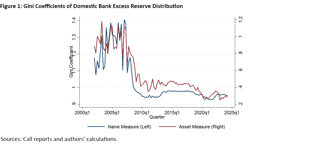
Figure 1 shows how the two measures have trended over the past two decades. Our new metric has been decreasing over the past few years, meaning that reserve balances have become steadily more evenly distributed. By contrast, the traditional Gini coefficient has actually been increasing during that same period. Our finding offers new insights into the evolving dynamics of reserve balances within the banking system.

Figure 1, line graph demonstrating the Gini Coefficients of domestic bank excess reserve distribution on a quarterly basis since Q1 of 2000. There are two lines: naive measure (left) and asset measure (right).

Enlarge

What Is the (Traditional) Gini Coefficient?

The Gini coefficient is a traditional measure of inequality. It quantifies the share of the area below the 45-degree line (the line of perfect equality) that lies above the Lorenz curve, as illustrated in Figure 2.

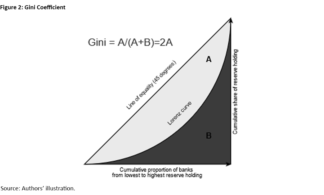
Figure 2, graph showing the Gini Coefficient. Gini = A/(A + B) = 2A.

Enlarge

The Lorenz curve illustrates the distribution of a variable (such as income, wealth or reserve balances) across all members of a group. In our context, the Lorenz curve plots the cumulative percentage of reserves against the cumulative percentage of banks. The traditional Gini coefficient ranges from zero (perfect equality) to 1 (maximum inequality).

Perfect Equality

If reserves are distributed evenly among banks, the Lorenz curve aligns with the 45-degree line. In this case, the area between the Lorenz curve and the 45-degree line is zero, resulting in a Gini coefficient of zero.

Greater Inequality

As the Lorenz curve moves farther from the 45-degree line, the area between the two increases. This leads to a higher Gini coefficient, reflecting greater inequality.

Maximum Inequality

In the most extreme case, where one bank holds all the reserve balances, the Lorenz curve remains flat and stays with the y-axis before jumping vertically once it reaches the x-axis. Here, the Gini coefficient reaches its maximum value of 1.

Why Weight the Gini Coefficient by Bank Assets?

To understand the need for asset-weighting Gini coefficients, consider this analogy: Suppose we want to measure income inequality of regions A and B. We could compare their GDPs, but identical GDPs do not imply equality. For instance, if A has double the population of B, then A would need about double the GDP for equality to hold. Measuring GDP differences without accounting for population size would exaggerate inequality.²

Similarly, banks differ in size, and this must be recognized when measuring inequality in reserve balances. Larger banks naturally hold more reserves due to higher reserve requirements, greater payment demands or larger investment portfolios. Treating all banks equally — as the traditional Gini coefficient does — artificially inflates inequality, and this is especially true for the U.S. banking sector considering the size differences among banks. For example, Figure 1 demonstrates that once we control for the reserve requirements and measure reserve balances in excess of reserve requirements, the upward trend of the traditional Gini coefficient reverses downward.³

Returning to the earlier analogy, GDP per capita is a more appropriate measure for measuring income inequality of regions, as it accounts for population differences. Also, an appropriate Gini coefficient should count every individual rather than each country. It means we should use population-weighted measures on the Lorenz curve. This approach yields the same total GDP, but weighing each country by population allows the Gini coefficient to better capture inequality. In our simple example of regions A and B, a population-weighted Gini coefficient is one-sixth, while the traditional Gini coefficient is zero.

The same logic suggests that we should measure bank size by asset amount, measure reserves per assets and derive the Lorenz curve with the asset-weighted measure. This results in the asset-weighted Gini coefficient. This approach accounts for the size of each bank by measuring reserves per unit of assets but preserving the total reserves in the banking system. The asset-weighted Gini coefficient ensures a more accurate representation of reserve inequality.

The following table compares the definition of the two Gini coefficients. Adjusting both the Gini-coefficient formula and the Lorenz curve with the asset-weighted measure, f(z), is crucial to preserve the property that the Gini coefficient is always between zero and 1.⁴

**Table 1: Gini Coefficient Definitions**
	Traditional Gini	Asset-weighted Gini
Formula	$1 - 2 \sum_{𝒴 i} L (𝒴 i) ƒ (𝒴 i), for increasing 𝒴_{i}$
Lorenz curve	$L (𝒴 i) = \frac{\sum_{𝒴 \leq 𝒴 i} 𝒴 ƒ (𝒴)}{\sum 𝒴 ƒ (𝒴)}$
𝒴_i =	bank i's reserves	$\frac{bank i's reserves}{bank i's assets}$
ƒ(𝒴_i) =	1	bank i's assets

Applying the Asset-Weighted Gini Coefficient

Having established the logic of the asset-weighted Gini coefficient, let us apply it to measure reserve inequality among U.S. domestic banks.

Figure 3 shows the trends in asset-weighted and traditional Gini coefficients from 2001 to 2023. Before the 2008 financial crisis, the asset-weighted Gini coefficient hovered around 0.62 but declined to about 0.32 after 2020. Conversely, the traditional Gini coefficient rose over the same period, from 0.87 precrisis to 0.95 post-2020.

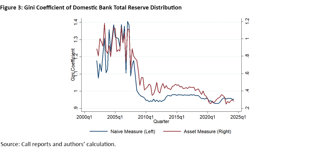
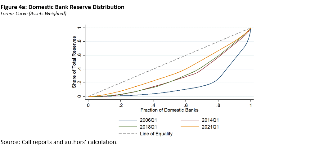
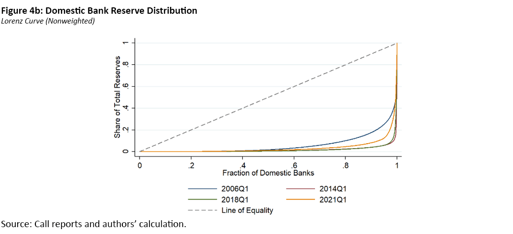
Figure 3, line graph demonstrating the Gini Coefficient of domestic bank total reserve distribution on a quarterly basis since Q1 of 2000. There are two lines: naive measure (left) and asset measure (right).

Enlarge

Figure 4 illustrates the corresponding Lorenz curves over time. The Lorenz curves behind the asset-weighted Gini coefficient have shifted closer to the 45-degree line, indicating increasing equality in reserve distribution. In contrast, the Lorenz curves for the traditional Gini coefficient have moved further from the 45-degree line, reflecting growing reserve inequality.

Figure 4a, line graph demonstrating the domestic bank reserve distribution with the Lorenz Curve (assets weighted). There are 5 lines: 2006 Q1, 2018 Q1, 2014 Q1, 2021 Q1, and line of equality.

Enlarge

Figure 4b, line graph demonstrating the domestic bank reserve distribution with the Lorenz Curve (nonweighted). There are 5 lines: 2006 Q1, 2018 Q1, 2014 Q1, 2021 Q1, and line of equality.

Enlarge

These trends align with the figures in Figure 3, revealing key patterns when we consider the following stylized findings about U.S. banks.

Larger Banks, Fewer Relative Reserves

Larger banks hold fewer reserves per unit of asset compared to smaller banks. For instance, before the 2008 crisis, the top five banks held about 40 percent of reserve balances but accounted for roughly half of total bank assets.

Quantitative Easing

Quantitative easing (QE) increases reserves per asset, with larger banks benefiting more. Regression analysis shows that QE amplified reserve differences between large and small banks, raising traditional Gini coefficients. However, the trend reversed after quantitative tightening began in 2019.

Large Bank Growth

Larger banks have grown faster than smaller banks in asset size. This trend was particularly pronounced from 2008 to 2010 due to mergers, acquisitions and the exits of smaller banks.

Conclusion

These findings are important in understanding the dynamics of reserve inequality. Our finding on QE explains why the traditional Gini coefficient rose during QE, as larger banks increased their shares of total reserves. It also clarifies the decline in traditional Gini coefficients post-2019 during quantitative tightening. And our finding on the growth of larger banks supports the long-term rise in traditional Gini coefficients, as larger banks' growing asset sizes naturally lead them to hold more reserves.

However, our finding on the relative reserve levels of smaller and larger banks reminds us that larger banks actually hold fewer reserves than smaller banks, after controlling for their size. Combining this with our other findings suggests that QE and the outgrowth of large banks have narrowed the (asset-weighted) inequality in reserves between large and small banks.

Thus, the asset-weighted Gini coefficient decreases over time, even as the traditional Gini coefficient increases. This divergence highlights the importance of using the correct measurement to capture inequality dynamics accurately.

Russell Wong is a senior economist in the Research Department at the Federal Reserve Bank of Richmond. Mengbo Zhang was a former dissertation intern at the Federal Reserve Bank of Richmond. We are thankful for comments from RC Balaban, Huberto Ennis, Anna Kovner and Alex Wolman.

For example, see the 2020 paper "Monetary Stimulus and Bank Lending" by Indraneel Chakraborty, Itay Goldstein and Andrew MacKinlay and the 2024 paper "The Reserve Supply Channel of Unconventional Monetary Policy" by William Diamond, Zhengyang Jiang and Yiming Ma.

This issue is well recognized in development economics.

Note that banks' excess reserve balances can be negative. As a result, their Gini coefficients (regardless of asset-weighting) can be greater than 1. In this case, the accumulating fraction of excess reserves runs below zero. This situation was more common before the 2008 financial crisis, when many banks (especially large ones) occasionally held negative excess reserves. In this case, the area between the 45-degree line and the Lorenz curve is greater than the area below the 45-degree line. Thus, its Gini coefficient is greater than 1, consistent with the time series plotted in Figure 1.

⁴

Without adjusting the Lorenz curve with the asset-weighted measure, the Lorenz curve could lay above the 45-degree line, for example, as in the 2015 paper "Large Excess Reserves in the United States: A View From the Cross-Section of Banks" by Huberto Ennis and Alexander Wolman.

Going Beyond: Additional Measures to Understand Reserve Demand

While the asset-weighted Gini coefficient offers some valuable insights into reserve distribution, it only captures part of the story. The following measures are complementary to fully grasp the dynamics of banks' demand for reserves:

Asset-Weighted Gini Coefficient

Purpose: Measures the distribution of reserves across banks, adjusted for their size
Insight: Helps identify inequality in and evolution of reserve holdings

Overnight Reverse Repo (ON RRP)

Purpose: Indicator of reserve abundance

Since the interest rate on reserves is higher than the ON RRP rate, market participants (such as money market mutual funds) prefer lending their excess liquidity to banks via repos rather than parking it at the Fed's ON RRP facility.
However, if banks already hold abundant reserves and demand no further borrowing, participants turn to ON RRP instead.
Thus, the volume of ON RRP signals how abundant reserves are in the system.

Caveat: The demand for ON RRP is also influenced by other factors, such as the supply of short-term government bonds. For more insights, see the 2021 article "The Borrower of Last Resort: What Explains the Rise of ON RRP Facility Usage?"

Reserve Demand Elasticity (RDE)

Definition: Measures the sensitivity of the (federal funds) borrowing rate to changes in the quantity of reserves banks borrowed (federal funds purchased)

High RDE: Indicates a shortage of reserves, with banks willing to pay higher prices to borrow additional reserves

Measurement Approaches:

Empirical: High-frequency federal funds market reports — such as the RDE measure produced by the New York Fed — can provide daily monitoring of RDE.
Structural: Our research adopts a model-based approach to estimate the long-run RDE over the last two decades, incorporating how frequently banks trade in federal funds markets. This is particularly useful for correcting selection bias, as banks alter or suspend their participation in the federal funds market over time.

To cite this Economic Brief, please use the following format: Wong, Russell; and Zhang, Mengbo. (May 2025) "How Concentrated Is the Distribution of Banks' Reserve Balances?" Federal Reserve Bank of Richmond Economic Brief, No. 25-18.