Skip to Main Content

Measuring Income Inequality and Economic Mobility

Econ Focus
First Quarter 2016
District Digest

Measures of income inequality and economic mobility have been gaining the public's and policymakers' attention in recent years. This is due, in part, to a long-run trend of increasing income inequality in the United States since 1979. According to recent data from the Congressional Budget Office (CBO), after-tax average household income for the poorest 20 percent of the population grew by 46 percent from 1979 to 2013, while the middle 60 percent saw a gain of only 41 percent over this period. The trend is even more striking with regard to the so-called "1 percent": From 1979 to 2013, the CBO reported growth in household income of 192 percent for the top 1 percent of households.

It seems likely that the fast growth of income accruing to the top 1 percent of households has sharpened the focus on income inequality. These figures do not necessarily translate into impoverishment for those at the lower end, however: Despite the growing disparity in income among households, average household income, adjusted for inflation, has grown across all of the commonly reported income groups reported by the CBO analysis.

The interest in income inequality may also stem from more recent economic trends that have included relatively healthy growth in employment accompanied by only modest gains in average wages. For example, while employment has grown an average of 1.6 percent nationally per year from 2010 to 2015, real wages have grown by only 0.8 percent over the same period. (See "Will America Get a Raise?") These trends are particularly important because labor income accounts for a larger share of income for households in the middle 60 percent of the distribution, ranging from 75 to 82 percent of average market income (that is, income from sources other than government transfer programs). In contrast, the poorest one-fifth of households earned 66 percent, and the richest one-fifth earned 65 percent, of their income as labor income in 2013.

Measuring Income Inequality

Assessing the changes in income distribution in the nation, or in states or metro areas, starts with an understanding of how the different government data sources define income. Common data sources include statistics drawn from tax return data available from the Internal Revenue Service (IRS), the U.S. Census Bureau's "money income" series, and estimates from the CBO — but there are important differences.

Starting with the narrowest definition, the IRS measures pretax income derived from federal tax return data. While these data have the advantage of more complete coverage for the highest-income households, and therefore are favored for reviewing trends of the top 1 percent, they suffer from the exclusion of important government transfers and under-representation at the bottom of the distribution because many families are not required to file tax returns. The Census data include pretax household income plus government cash transfers such as Social Security, unemployment insurance, and cash public assistance. These additional elements of income tend to disproportionately benefit households at the lower end of the distribution. Finally, the broadest measure is the net after-tax income data provided by the CBO, which use more detailed tax record information combined with demographic characteristics and income data from the Census, but also include government transfers as well as capital gains income and some imputed noncash sources of income, and subtract direct and indirect federal taxes. These different measures can generate somewhat different conclusions about the trends in income inequality — for the magnitude of change, if not the direction.

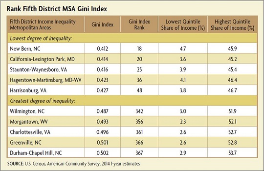
The standard measure of income inequality is the Gini index (sometimes called the Gini coefficient). The Gini index, developed in the early 20th century by Corrado Gini, summarizes the entire distribution of income in a single metric ranging from zero to one. A Gini index of zero would result if income were distributed equally across all groups, while a value of one indicates that all of the income is received by the highest-income group, with none going to the lower-income groups. This metric can be used to compare a single region over time or to compare geographic units such as states or countries.

The Gini index calculated from the CBO's broader definition of net after-tax income is lower than the same index based on before-tax income. Even so, the trend over time is very similar between the different measures. In 1979, the Gini index based on after-tax income was 0.36, but by 2013, it had risen to 0.44. The effect of government transfers and the progressivity of the federal tax system help to reduce income inequality. The Gini index on market income, which excludes these effects, was 0.60 in 2013. This higher value (more unequal distribution of income) is similar to estimates that economists have generated on pretax measures of income derived from federal income tax return data. (See chart below.)

Another way to determine how the distribution of income is changing is to examine directly the shares of income going to equally sized groups of households. Typically, the data are reported for quintiles of households, where households are ranked from lowest to highest household income. The lower quintile represents the poorest 20 percent of households, while the highest quintile represents the richest 20 percent of households. This view of the data from the CBO also offers additional detail on the top quintile, including a breakout of the top 1 percent.

While the somewhat narrower definition of income used by the Census also provides income shares by quintiles and the top 5 percent, it does not have enough detail at the higher end to report on the top 1 percent of the distribution. The 95/20 percentile ratio, however, is often used to describe how far the top 95 percent of the income distribution is from the lower quintile. In the most recent data for 2014, this ratio was 9.64, meaning that the income at the 95th percentile was 9.64 times the income at the 20th percentile. In 1979, it was markedly lower, at 6.69, reflecting the fact that household income rose faster from 1979 to 2014 for households in the 95th percentile than it did for the lower quintile of the household income distribution.

Measuring Economic Mobility

While the income distribution in any given year is a snapshot in time, generally we think of economic mobility as the opportunity to move along the income ladder, either in one's own life or across generations. The Richmond Fed's 2012 Annual Report featured an essay by Kartik Athreya and Jessie Romero on economic mobility that suggested that for most people, mobility depends on opportunities to obtain human capital. Individuals have differing abilities and preferences that may ultimately determine their outcomes, however, making it problematic to equate equality of outcomes with equality of opportunity.

As with income inequality, economic mobility can be measured in various ways. The data required to measure economic mobility present some challenges, as individuals need to be tracked over time. Intragenerational mobility measures the movement of an individual along the income distribution during his or her own lifetime. Income typically rises through the prime working-age years and then declines during retirement, but positive and negative shocks can occur as well. Intergenerational mobility, perhaps a more interesting view, compares the outcome of an individual with the outcome of his or her parents at the same stage of life (say 40 years of age). Intergenerational mobility can be measured either in absolute terms — does the child earn a higher income than his or her parent did at the same age? — or in relative terms — is the child's income rank higher than that of his or her parent?

In absolute terms, most people have been upwardly mobile compared to their parents. The Economic Mobility Project (Pew Charitable Trusts) reported in their 2012 analysis of the Panel Study of Income Dynamics that 84 percent of U.S. adults earned a higher family income than their parents at a comparable age. The study compared parents' income, measured from 1967 to 1971, to the income of their children, who were tracked into adulthood to an average age of 45 during the period from 2000 to 2008.

More recent research has focused on relative intergener­ational income mobility. Intergenerational mobility trends can be presented in several ways. A standard approach is to sort children and their parents into their respective income quintiles and to plot the results into what is termed a social mobility transition matrix. The intergenerational elasticity of earnings (IGE) is another commonly used form of analysis, resulting in a single summary metric that can be used for comparison across time, across demographic characteristics, or across geographies. The IGE estimates the relationship between parental and child incomes around age 35 or 40 and describes, in percentage terms, how much of the difference in earnings in one generation persists into the next generation. A smaller IGE suggests less persistence in inequality and greater mobility. Estimates have found that the United States has relatively low economic mobility compared to other countries, with an IGE around 0.5 or 0.6 compared to 0.2 to 0.3 for Canada and some of the Nordic countries. In addition, studies suggest that intergenerational mobility declined in the United States between 1980 and 1990 and has since been fairly constant.

Trends in Income Inequality and Economic Mobility

The relationship between income inequality and economic mobility has sparked debate among economists. There appears to be a negative correlation between income inequality, represented by the Gini index, and economic mobility, as measured by the IGE, when comparing countries. This relationship was dubbed the "Great Gatsby" curve in a 2012 speech by Alan Krueger, who used the correlation to sound an alarm about the prospects for deteriorating economic mobility in the future given that income inequality has worsened in recent decades and economic mobility outcomes for the next generation will not be known for some time.

Of course, correlation between income inequality and economic mobility does not imply causality; there are a host of other potential factors influencing economic mobility, including family structure and investments in early education. New research being conducted by the Brookings Institution (in partnership with the Urban Institute and Child Trends) is using a model called the Social Genome Model (SGM) to focus on the dynamic movement from one stage of life to the next. An important feature of the model is that it allows for simulations of policy interventions at any stage so that the impact on outcomes at subsequent stages can be measured. The SGM starts with a child's circumstances at birth and then estimates the probability of success at each stage starting with early childhood, where success is measured by acceptable pre-reading and math skills and behavior that is generally school appropriate. Other stages include middle childhood, adolescence, transition to adulthood, and finally adulthood, where success is defined as reaching middle class. The SGM is just one example of the types of models and new datasets that researchers are using to explore the factors that influence both income inequality and economic mobility.

Income Inequality and Economic Mobility in the Fifth District

When it comes to measures of income inequality and economic mobility, the states in the Fifth District vary widely. Using the Gini index as a measure of income inequality, Maryland had the least inequality in income, with a Gini index of 0.449, while the District of Columbia had the greatest income inequality, with an index of 0.522, based on Census data for 2014. All of the states in the Fifth District had a Gini index lower than the 0.48 index for the nation, but the District of Columbia had greater inequality than all 50 states. (See table below.)

The Census provides a Gini index for 381 metropolitan areas in the United States, with 46 of those areas located within the Fifth District. Most of the metropolitan areas within the Fifth District had lower income inequality than the nation as a whole, and for many of the metropolitan areas with a higher Gini index, the value was not statistically different from the U.S. index. In fact, of the Fifth District metropolitan areas, only the Durham-Chapel Hill, N.C., metropolitan area had income inequality that was statistically more unequal than the nation. (See table below.)

For many metropolitan areas, income inequality has increased in recent years, as it has in the nation. A recent Brookings Institution analysis of the change in income inequality from 2007 to 2014 in the country's 100 largest metropolitan areas found that several Fifth District metropolitan areas experienced a statistically significant increase in inequality over this period as indicated by an increase in the 95/20 ratio. These included Charlotte, N.C.; Raleigh, N.C.; Washington, D.C.; and Virginia Beach-Norfolk, Va. None of the Fifth District metro areas included in the Brookings analysis experienced a decline in inequality.

These findings must be qualified, however. The smaller sample size for metropolitan areas, even the largest 100, introduces more error around the estimates, which means some of the movement, both positive and negative, does not reliably indicate a change. In addition, as noted earlier, the Census definition of income, which is the primary source for states and metro areas, does not include all of the effect of government transfers and the federal tax system that is used by the CBO to calculate net after-tax income. These adjustments to money income generally serve to improve outcomes for the lower quintiles and lower net income for the upper quintiles.

Exploring the differences in economic mobility across geographic areas is difficult because the measures that have become the standard at the national level, the IGE and the transition matrix, are not easily replicated at the regional level due to data constraints. Research at the Pew Economic Mobility Project provides state-level analysis of economic mobility using earnings data from the Survey of Income and Program Participants as well as the Social Security Administration's Master Earnings File. In combination, these datasets allow researchers to examine intragenerational mobility, using a 10-year span between ages 35-39 and 45-49.

Pew researchers calculated two measures: (1) absolute mobility, measured as the growth in earnings between the two five-year periods; and (2) relative mobility, or the change in an individual's percentile rank in the earnings distribution over the 10-year period. For the relative mobility measure, upward mobility was defined as a movement from the bottom half of the earnings distribution at age 35-39 to 10 or more percentage points higher in the distribution by age 45-49. Similarly, downward mobility was measured as movement from the top of the income distribution (above the median) at age 35-39 to 10 or more percentiles lower in the earnings distribution by age 45-49. Relative mobility was calculated using the national earnings distribution as well as the regional earnings distribution, although the discussion that follows references only the national earnings distribution.

In these results, Maryland was the only state where relative upward mobility was higher than the national average, while three states in the Fifth District — North Carolina, South Carolina, and Virginia — had upward mobility rates that were below the national rate. Maryland was also the only state in the District with absolute mobility that was significantly higher than the national average. Rates of downward mobility for the District reveal that Maryland and Virginia both had rates of relative downward mobility that were better (that is, lower) than the national average. (See table below.)

To explore economic mobility across metropolitan areas in the Fifth District, we turn to work done by Raj Chetty of Stanford University and co-authors using yet another measure of economic mobility, one that relies on data from tax records. In order to reveal differences across geographic areas within the United States, their work focused on commuting zones that cover the entire country, although they also calculated their measures for counties and metropolitan areas. Instead of calculating the IGE, the authors use a "rank-rank" measure that describes the correlation between the parents' rank in the national distribution and the children's rank. As with the measure used in the Pew study, Chetty and co-authors also calculate an absolute upward mobility measure that generates the expected rank of children whose parents are at the 25th percentile of the national income distribution. Broadly speaking, mobility appears to be lowest in the Southeast and highest in the Midwest.

Interestingly, within the Fifth District, we see the same pattern emerge if we look at the measure of absolute upward mobility for metro areas — the lowest values are primarily in North and South Carolina and in the Virginia Beach-Norfolk metro area, while higher values, and therefore higher expected income ranks, are measured for metro areas in the northern and western part of the District. (See map below.) The authors explore many factors that may help to explain geographical differences in economic mobility, including race, segregation, inequality, school quality, social networks, and family structure. They stop short of identifying which of the factors is the most important determinant of upward mobility but provide plenty of data and questions to be addressed in future research.

The available data indicate that the United States has become a nation with greater income inequality since 1979 and relatively flat economic mobility since 1990. Although there is no causal relationship between income inequality and economic mobility, some economists have raised concerns about the underlying factors that seem to influence both trends. Within the Fifth Federal Reserve District, every state had lower inequality than the national average, while the District of Columbia had the highest level of inequality in the country.

Subscribe to Econ Focus

Receive an email notification when Econ Focus is posted online.

Subscribe to Econ Focus

By submitting this form you agree to the Bank's Terms & Conditions and Privacy Notice.

Phone Icon Contact Us

David A. Price (804) 697-8018