Can China Avoid a Liquidity-Trap Recession? Some Unintended Consequences of Macroprudential Policies

By Russell Wong

Economic Brief

April 2024, No. 24-12

Efforts to avoid a liquidity trap could ultimately cause one to happen. In this article, I examine how this occurs, what implications such actions have for other macroeconomic policies and what else can be done to avoid liquidity traps.

In Shakespeare's famous tragedy, Macbeth acknowledged his biggest threats and was determined to do whatever it took to prevent them. Fueled by ambition and overconfidence, he was ultimately trapped in a self-fulfilling tragedy: The draconian measures he used to avoid the downfall he feared only realized his downfall sooner. Like Macbeth, sometimes policymakers imposing heavy-handed measures to prevent a liquidity trap might find themselves in a similar self-fulfilling tragedy.

A liquidity trap is a recession featuring excessive savings such that the nominal interest rate of saving drops to its effective lower bound, which is typically zero. (If it were lower, people could hold cash instead to avoid negative nominal interest rates.) It features a spiral of deflationary pressure and economic slacks like high unemployment rates and GDP far below its potential, as seen in the Great Depression in the 1930s and the Great Recession in 2008.

A liquidity trap is a nightmare for central banks because the zero lower bound constrains them from further reducing the nominal interest rate to stimulate the economy. The nightmare can be long: For example, Japan — formerly the world's second-largest economy after the U.S. — has been battling its liquidity trap since its real-estate bubble burst in 1990. Recently, some commentators have argued that a liquidity trap is imminent in China — currently the world's second-largest economy — pointing to signs such as deposit surge (despite declining interest rates), mounting deflationary pressures and high unemployment rates among youth.

Avoiding Liquidity Traps

It is now widely accepted that a better way to fight a liquidity trap is to avoid it, which is the idea behind many macroprudential policies nowadays. For example, China has recently introduced various macroprudential policies — the so-called "three red lines" — to its real estate sector, bearing Japan's lessons in mind.¹

But how does a liquidity trap happen in the first place? We need to understand its mechanism to defuse it. In a traditional Keynesian analysis, a liquidity trap happens when the downward sloping investment-saving (IS) curve cuts the flat portion of the liquidity preference-money supply (LM) curve.

However, this account of a liquidity trap is found unsatisfactory in explaining Japan's balance-sheet recession in 1990 and the U.S.'s Great Recession in 2008. As pointed out by economist Richard Koo, the massive deleveraging of heavily indebted firms and households had a clear role in these two famous liquidity traps (and possibly even in China) but was not so clear in the IS-LM theory. Recent academic research has explicitly analyzed the role of deleveraging in a liquidity trap and its implication on policy.² In this article, I analyze the effect of a leverage regulation that aims to prevent a liquidity trap, based on my recent research. All the derivation can be found in the footnotes.

To analyze the consequences of (de)leveraging, consider the situation of borrowers and savers in an economy. Borrowers are typically firms, local governments or leveraged investors (such as those invested in real estate) that rely on rolling over previous debt (denoted as $d_{0}$ ) to continue their operations. Savers are typically households and investors who decide how much of today's income to save (denoted as $d^{S}$ ) to earn the interest rate $r$ for tomorrow's consumption.

As in standard economic analysis, savers choose the level of saving such that their intertemporal marginal rate of substitution ( $M R S$ ) between today's consumption and tomorrow's consumption equals the interest rate, denoted as $M R S^{S} (d^{S}) = r$ . The $M R S$ measures the marginal utility of today's consumption against the marginal utility of tomorrow's consumption (that is, the amount of tomorrow's consumption needed to gain per unit of today's consumption forgone to keep the total savers' utility unchanged).³ Since the saver's $M R S$ is increasing in the level of saving, it constitutes an upward sloping supply curve in the debt market, as illustrated in Figure 1.

Figure 1, line graph illustrating the determination of the interest rate and debt level with saving and borrowing on the x-axis and interest rate on the y-axis. There are two intersecting lines: the supply curve and the demand curve. Dotted lines mark the equilibrium interest rate and equilibrium debt level.

Enlarge

Similarly, the borrowers decide how much of their debt today (denoted as $d^{B}$ ) is rolled over to maintain today's consumption, which costs them interest and reduces tomorrow's consumption. Again, the borrowers choose the level of borrowing such that their $M R S$ equals the interest rate, denoted as $M R S^{B} (d^{B}) = r$ .⁴ Since the borrower's $M R S$ is decreasing in the level of borrowing, it constitutes a downward sloping demand curve in the debt market.

In equilibrium, borrowing equals saving equals the aggregate level of debt ( $d^{B} = d^{S} = d$ ) such that the debt market clears today, as illustrated in Figure 1. Of course, the same process will repeat tomorrow and so on. In the steady state, the interest rate equals the agent's rate of time preference, and the borrowers' debt will be rolled over indefinitely (shown as $d = d_{0}$ in Figure 1).⁵

Now, suppose an excessive aggregate level of debt also exposes the economy to the risk of a liquidity trap tomorrow. When a liquidity trap happens, the nominal interest rate falls to the zero lower bound, and output falls below its potential. Since my focus is the policymaker's response to excessive debt today (and ultimately the liquidity trap tomorrow), I leave out the details of how the probability of a liquidity trap is determined. What is important is that the likelihood of a liquidity trap tomorrow is zero when the aggregate level of debt today is below some threshold (i.e., $d \leq θ$ ). Otherwise, it is increasing in the aggregate level of debt. A relevant case is when borrowers are heavily indebted such that the inherited debt is greater than the threshold (that is, $d_{0} > θ$ ).

To eliminate the liquidity trap tomorrow, policymakers impose a leverage regulation on borrowers today: Their choice of debt cannot exceed some debt limit $\overline{d}$ in any period (that is, $d^{B} \leq \overline{d}$ ) where $\overline{d} \leq θ$ . Since borrowers have inherited excessive debt ( $d_{0} > θ$ ), the leverage regulation forces them to deleverage today, following the premise that $d^{B} \leq \overline{d} \leq θ < d_{0}$ .

The leverage regulation considered above is found in many macroprudential policies. For example, Basel III imposes a similar leverage ratio requirement on banks. Regulators impose leverage regulations on non-financial firms as well. For example, China recently set restrictions on giant but highly leveraged real estate developers to stop further unchecked expansion of debt. The leverage of these developers has stalled since then.

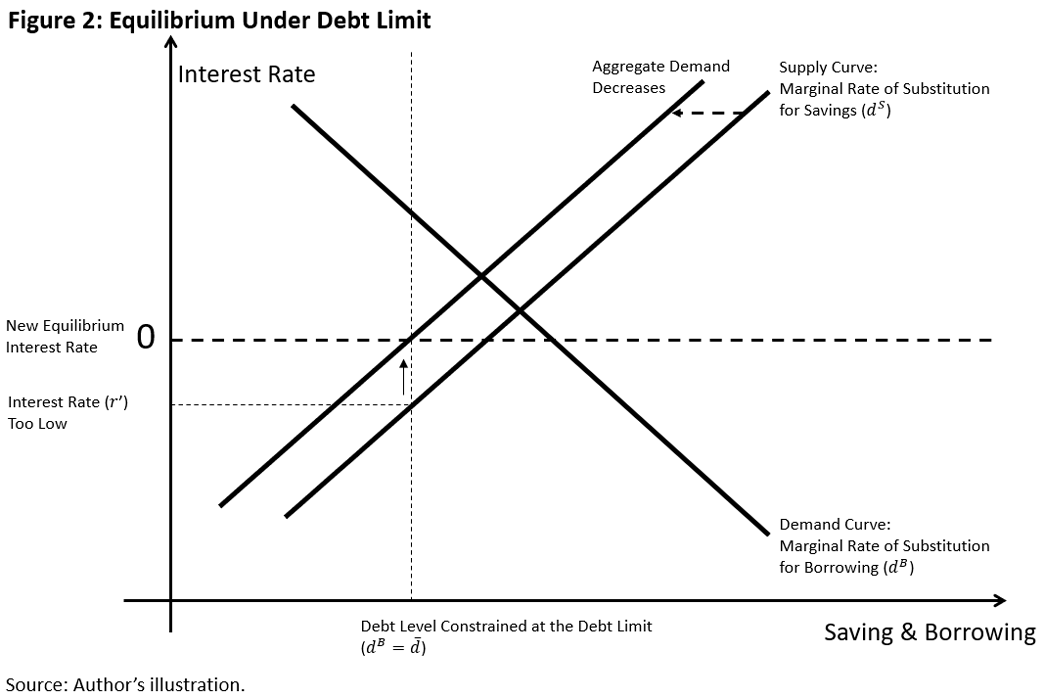
What will be the consequence of imposing the leverage regulation? One can construct the new equilibrium as illustrated in Figure 2. In the new equilibrium, the interest rate equals savers' $M R S$ with their level of saving at the debt limit in every period (that is, $r^{'} = M R S^{S} (\overline{d})$ ).⁶ At this interest rate, savers are indifferent to making further savings beyond the debt limit. On the other hand, borrowers have a higher $M R S$ than this interest rate, so they want to borrow more but cannot because of the debt limit. As shown in Figure 2, the debt market under the debt limit clears at the lower interest rate $r^{'}$ . In this case, the leverage regulation with a low level of $\overline{d}$ eliminates the risk of a liquidity trap and prevents output from falling below its potential in the future. A low $\overline{d}$ is also desirable to provide some buffers when $θ$ is uncertain.

Figure 2, line graph illustrating the equilibrium under debt limit with saving and borrowing on the x-axis and interest rate on the y-axis. There are 3 intersecting lines: the supply curve, demand curve, and aggregate demand decreases. Dotted lines mark the new equilibrium interest rate, when the interest rate is too low, and when the debt level was constrained at the debt limit.

Enlarge

So far, so good, but only if savers' $M R S$ is always above the lower bound associated with the zero nominal interest rate. Note that the interest rate that clears the debt market is the real rate (or the nominal interest rate minus the expected inflation rate). For simplicity, consider that there is no inflation, so the real and nominal interest rates are the same. (Later, we will consider the general case.) Thus, there is a zero lower bound for the real interest rate.

What would happen if the leverage regulation is so restrictive that savers' $M R S$ is below the zero lower bound, as illustrated in Figure 2? Then, savers' marginal utility of consumption is much lower today than tomorrow. It could happen when the leverage regulation forces borrowers to abruptly deleverage their borrowing from $d_{0}$ to $\overline{d}$ . In equilibrium, it means savers also abruptly reduce their savings from $d_{0}$ to $\overline{d}$ to clear the debt market. This dissaving is achieved by a significant increase in savers' consumption today. Since the marginal utility of consumption is decreasing — thanks to the law of diminishing marginal utility — a higher level of today's consumption implies the marginal utility of consumption is much lower today than tomorrow (that is, a lower $M R S$ ). Thus, a restrictive leverage regulation featuring a low $\overline{d}$ can push the interest rate below the zero lower bound.

But the interest rate cannot be negative in equilibrium, so something else must be accommodated to restore the interest rate at the zero lower bound illustrated in Figure 2. Recall that the aggregate demand for output is the sum of savers' and borrowers' consumption. In normal times, if aggregate demand is below the potential output $\overline{Y}$ , the interest rate decreases to push aggregate demand back to the potential level (as savers save less and borrowers borrow more to consume), and vice versa.

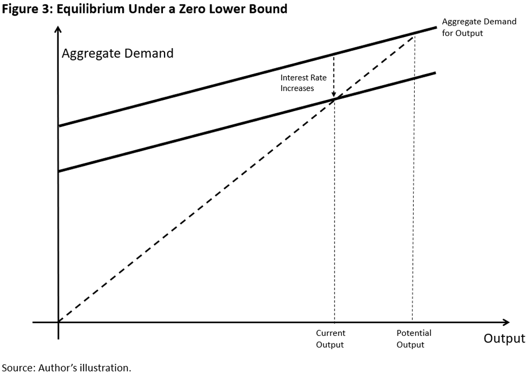
However, if the interest rate at the potential output level is already negative, the interest rate has to increase until it is restored at the zero lower bound and, hence, the aggregate demand decreases below the potential output level, as illustrated in Figure 3.

Figure 3, line graph illustrating the equilibrium under a zero lower bound with output on the x-axis and aggregate demand on the y-axis. There are two lines: the aggregate demand for output and the interest rate increases, with the current and potential output both marked with dotted lines.

Enlarge

What is the logic behind the aggregate demand curve in Figure 3? Since savers' $M R S$ is now stuck at zero, it dictates an autonomous level of savers' consumption today, denoted as $C^{S}$ .⁷ It is the level of today's consumption required to keep savers' savings at the zero lower bound.

On the other hand, borrowers' consumption is their income minus paying inherited debt plus rolling over new debt under the debt limit at the zero lower bound (that is, $C^{B} = Y - d_{0} + \overline{d}$ ). As an illustration, if savers and borrowers share the economy equally, the aggregate demand for output is simply $A D = 0.5 C^{B} + 0.5 C^{S} = 0.5 Y + 0.5 (C^{S} - d_{0} + \overline{d})$ .

In general, aggregate demand will be some weighted average between borrowers' and consumers' consumption, so aggregate demand is always flatter than the 45-degree line. At the zero-lower-bound equilibrium, aggregate demand equals the output (that is, $A D = Y$ ), cutting the 45-degree line below the potential output level, as illustrated in Figure 3.

Leverage Regulations and Liquidity Traps

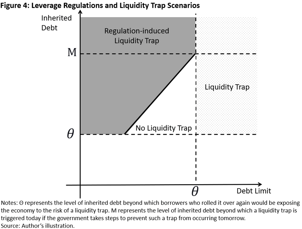
Thus, a restrictive leverage regulation designed to eliminate a liquidity trap tomorrow can lead to a liquidity trap recession today, fulfilling a Macbethian tragedy. Figure 4 illustrates the equilibrium over each regulation and leverage scenario:

Scenario 1: The leverage regulation can eliminate a liquidity trap in the white corridor where the inherited leverage is not too high and the leverage regulation is not too restrictive (moderate debt limit). The higher the inherited leverage, the narrower the corridor.
Scenario 2: If the leverage regulation is not restrictive enough (debt limit higher than θ in the dotted region), then the risk of a liquidity trap is not eliminated.
Scenario 3: If the leverage regulation is too restrictive (the shaded region), the leverage regulation also induces the economy into a liquidity trap.
Scenario 4: If the economy inherits too much leverage (higher than $M$ ), the corridor disappears, and no leverage regulation can prevent the economy from a liquidity trap by itself or by regulation.⁸ A Macbethian tragedy is inevitable in this region.

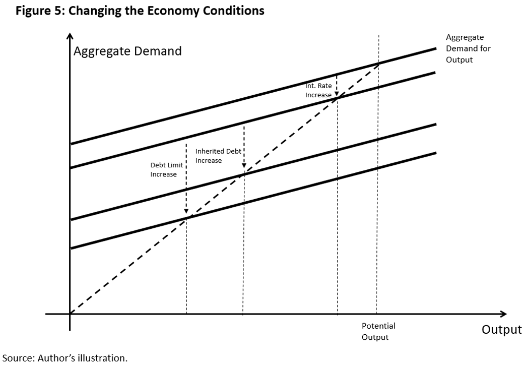
Figure 4, line graph illustrating leverage regulations and liquidity trap scenarios with the debt limit on the x-axis and inherited debt on the y-axis. Three different regions are shaded: liquidity trap, no liquidity trap, and regulation-induced liquidity trap.

Enlarge

A regulation-induced liquidity trap is more devastating (in terms of output) when the borrowers are more indebted (higher $d_{0}$ ) or the leverage regulation is more restrictive (lower $\overline{d}$ ). In these cases, the supply curve in Figure 2 shifts to the right, so a bigger reduction in output is needed to restore the supply curve at the zero lower bound. The multiplier effect on output by a higher $d_{0}$ or a lower $\overline{d}$ is illustrated by shifting the aggregate demand curve downward in Figure 3.

Note that a lower $\overline{d}$ has a larger multiplier effect than a higher $d_{0}$ , as illustrated in Figure 5. This is because a lower $\overline{d}$ reduces both borrowers' consumption (the part $\overline{d}$ in the aggregate demand, as they can borrow less) and savers' consumption (via $C^{S}$ implicitly, as their wealth is lower eventually), whereas a higher $d_{0}$ only reduces the former. A policy insight is that a restrictive leverage regulation is more devastating than the excessive leverage it regulates.

Figure 5, line graph illustrating the aggregate demand for output with changing economy conditions. Output is on the x-axis and aggregate demand is on the y-axis. The debt limit increase, inherited debt increase, and interest rate increase are marked with dotted lines.

Enlarge

Implications for Fiscal Policies

A liquidity trap induced by leverage regulation has different policy implications, too. A typical prescription from Keynesian IS-LM theory is that fiscal stimuli — such as government spending and transfers — are powerful during the liquidity trap as they shift the IS curve up without the crowding out effect from raising the interest rate. Another popular narrative for fiscal transfers is that they encourage consumption among cash-constrained consumers and boost aggregate demand toward the potential output.

In the regulation-induced liquidity trap, however, fiscal transfers will have limited effects for three reasons.

High Interest Rates

First, savers consume little in the liquidity trap not because they are cash constrained but because — even if nominal interest rates are low — the real interest rate is so high that they prefer saving to consumption. So, any fiscal transfers to the savers will mostly be saved rather than consumed. Consumption-based transfers like consumption vouchers might work, but agents can always substitute cash purchases with the vouchers without raising their consumption much.

Taxes

Second, if the fiscal transfers are financed by raising public debt (which is ultimately paid for by future taxes), agents will save the transfers for the future tax payment: the logic of Ricardian equivalence. Essentially, debt-financed transfers are like forced borrowings: borrowing the transfers today and paying back the transfers plus taxes tomorrow. Thus, the savers' supply curve in the debt market in Figure 2 shifts to the right (from saving the transfers) but is completely absorbed by the increased government debt. Thus, the net supply curve is the same.

Market Frictions

Third, note that Ricardian equivalence holds if the debt market is complete and frictionless, which is the case for savers but not the case for borrowers due to the debt limit. So, in principle, transfers to borrowers would increase their consumption since they have a higher marginal propensity to consume and always want to leverage to consume but cannot. However, this channel only works because debt-financed transfers are essentially borrowing without being subject to the debt limit. If the tax obligations were counted toward the debt limit, then the stimulus effect of the borrowers would be gone.

In other words, transfers to borrowers could stimulate aggregate demand, but only because it indirectly reduces the debt limit. Therefore, the root of the stimulus effect is still the restrictive leverage regulation.

Fiscal Transfer Multipliers

What will be the multiplier of the fiscal transfers during a regulation-induced liquidity trap? In this case, borrowers will consume all the transfers, so we have $C^{B} = Y - d_{0} + \overline{d} + T$ , where $T$ is the amount of the debt-finance transfers to borrowers and savers. Ricardian equivalence implies that the savers' consumption $C^{S}$ is the same. Summing these two, the aggregate demand curve shifts up in Figure 5. If savers have a bigger share of the economy, the aggregate demand curve will be flatter, the shift up will be lower, and hence the multiplier will be smaller (and it would equal 1 when savers and borrowers have equal shares).

In sum, fiscal transfers will have limited effects on output during a regulation-induced liquidity trap. Nevertheless, large enough transfers can lift the economy out of the liquidity trap, despite not being very effective. Of course, it would be easier to lift the economy by relaxing the leverage regulations. But when rolling back the leverage regulations is not an option (for example, in the Macbethian tragedy scenario), fiscal transfers could be the next-best option.

What's Next?

Back to China: Containing excessive leverage — as is the goal of any macroprudential policy — is generally right for minimizing the risk of a liquidity trap. This article highlights the narrow corridor of regulating excessive leverage: Imposing too-restrictive leverage regulation will only make the liquidity trap more likely.

Bearing this in mind, what should we pay attention to next? Based on the above analysis, let's conclude with the following scenarios that would make a liquidity trap more likely.

Pessimism: Pessimistic households and investors more concerned about China's downside risks will save more. This would shift down both the aggregate demand curve (lower $C^{S}$ ) and the supply curve in the debt market (lower $M R S$ ).
Deflation expectations: Expecting deflation would raise the lower bound for the real interest rate in the debt market. A larger output gap is thus needed to maintain the interest rate at the lower bound (lower $C^{S}$ ), which adds to the deflation pressure and fulfills the deflation expectation.
Collapse in real estate prices: If real estate properties are pledged as collateral, a price collapse will trigger a forced deleverage.
Bank runs: On top of widening the output gap, bank runs would also reduce the supply of savings to maintain the interest rate at the zero lower bound.

Russell Wong is a senior economist in the Research Department at the Federal Reserve Bank of Richmond.

For a historical review of China's financial policies, see the 2020 paper "Macroeconomic Effects of China's Financial Policies" by Kaiji Chen and Tao Zha.

For example, see the 2012 paper "Debt, Deleveraging and the Liquidity Trap: A Fisher-Minsky-Koo Approach" by Gauti Eggertsson and Paul Krugman, the 2016 paper "Liquidity Trap and Excessive Leverage" by Anton Korinek and Alp Simsek and the 2016 paper "A Theory of Macroprudential Policies in the Presence of Nominal Rigidities" by Emmanuel Farhi and Ivan Werning.

To be precise, the saver's $M R S$ is given by: $M R S^{S} (d^{S}) = \frac{U^{'} [Y + d_{-1}^{S} - d^{S} / (1 + r)]}{U^{'} [Y + d^{S} - d_{+1}^{S} / (1 + r_{+1})] / (1 + ρ)} - 1$ , where $U^{'} (C)$ is the marginal utility of consumption, $Y$ is income, $ρ$ is the rate of time preference and the subscripts of " $+1$ " and " $-1$ " denote the variables in the next and previous periods, respectively. The saver's consumption is $C^{S} = Y + d_{-1} - d^{S} / (1 + r)$ today and $C_{+1}^{S} = Y + d^{S} - d_{+1}^{S} / (1 + r_{+1})$ tomorrow.

⁴

Similarly, the borrower's $M R S$ is given by: $M R S^{B} (d^{B}) = \frac{U^{'} [Y - d_{-1}^{B} + d^{B} / (1 + r)]}{U^{'} [Y - d^{B} + d_{+1}^{B} / (1 + r_{+1})] / (1 + ρ)} - 1$ .

⁵

In the steady state, we have $d_{+1}^{S} = d_{+1}^{B} = d = d_{0}$ , Since $d_{0}^{S} = d_{0}^{B} = d_{0}$ , substituting this equality in the definition of $M R S$ , we have $r_{+1} = r = ρ$ .

⁶

Note that the saver's $M R S$ under the leverage regulation becomes: $M R S^{S} (\overline{d}) = \frac{U^{'} [Y + d_{0} - \overline{d} / (1 + r)]}{U^{'} [Y + ρ \overline{d} / (1 + ρ)] / (1 + ρ)} - 1 end entire equation$ .

⁷

In particular, $C^{S}$ solves $U^{'} (C^{S}) = U^{'} [Y + ρ \overline{d} / (1 + ρ)] / (1 + ρ)$ .

⁸

To be precise, $M = C^{S} - Y + θ / (1 + r)$

To cite this Economic Brief, please use the following format: Wong, Russell. (April 2024) "Can China Avoid a Liquidity-Trap Recession? Some Unintended Consequences of Macroprudential Policies" Federal Reserve Bank of Richmond Economic Brief, No. 24-12.

This article may be photocopied or reprinted in its entirety. Please credit the author, source, and the Federal Reserve Bank of Richmond and include the italicized statement below.

Views expressed in this article are those of the author and not necessarily those of the Federal Reserve Bank of Richmond or the Federal Reserve System.