How Seasonality in Inflation Variance Affects Estimates of Underlying Inflation

The Federal Reserve has a mandate to achieve price stability, which it interprets as inflation that averages 2 percent over time. Retrospectively, it is simple to determine how successful the Fed has been in achieving this goal. In real time, however, a key challenge for the Fed is inferring the current level of "underlying" inflation, as that involves filtering out the noise from volatile monthly inflation data. In this article, we show that there is a seasonal aspect to the volatility of PCE inflation that makes it desirable (and important) to filter differently depending on the month of the year.

Why Examine Seasonality in Variance in Inflation

Recent work has studied residual seasonality in inflation.¹ Standard seasonal adjustment procedures are aimed at seasonality in the level of a data series. The work on residual seasonality has been concerned with the possibility that those adjustment procedures may not have captured some recent seasonal patterns, allowing them to flow through to seasonally adjusted data. This article is instead focused on seasonality in variance, which traditional adjustment procedures do not address.² We work with seasonally adjusted data; to the extent that there is residual (level) seasonality in that data, we are not addressing it. Rather, our focus is on how inference about underlying inflation should consider seasonality in variance.

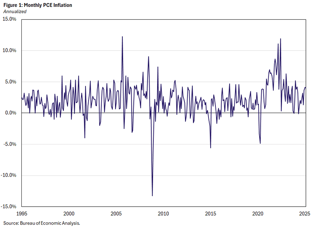
The FOMC has a 2 percent target for PCE inflation. At the end of each month, the Bureau of Economic Analysis publishes PCE inflation as part of its Personal Income and Outlays report. Figure 1 displays the monthly PCE inflation rate, converted to an annualized rate of change. Monthly inflation is highly volatile, so determining whether its behavior is consistent with the target — that is, inferring the current level of underlying inflation — is not simple.

There are many complementary methods for inferring the level of underlying inflation. Some use information in the Personal Income and Outlays report covering the entire distribution of price changes. With these methods, inflation movements that can be attributed to large price changes for a small share of expenditures are down weighted relative to more broad-based movements.³

Other methods use only the information in inflation itself.⁴ These univariate methods — the focus of this article — are generally based on the idea that the monthly inflation rate we observe is the sum of a trend (underlying inflation) and noise. In turn, the trend is often assumed to be a random walk. That means that whatever our estimate of the trend is in a particular month, we expect it to remain at that level the next month, although next month we update our estimate based on the incoming data.

By estimating the relative volatility of the noise and the changes in trend, this approach provides a rule for updating our estimate of trend inflation each month based on the error in our forecast of actual inflation. The rule specifies that the larger the estimated variance of the noise (compared to the change in trend), the less we update our estimate of the trend in response to a given forecast error.

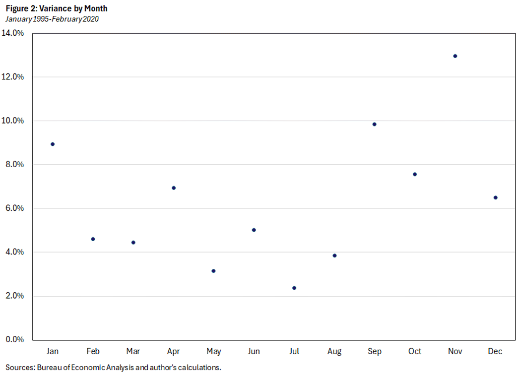
While the univariate methods often allow the variances to evolve over time — so-called "stochastic volatility" — they typically assume that the variances do not depend on the month of the year. Figure 2 displays the variance of monthly inflation, which differs substantially from month to month. This might seem odd because the data we are using is seasonally adjusted. But, as mentioned above, seasonal adjustment addresses only the level, not the volatility of a variable.

Modeling Seasonality in Variance

To accommodate the seasonal pattern in the variance of inflation apparent in Figure 2, we estimate a time-series model of PCE inflation that is a slight variation on the ones described above. The assumptions are as follows, with the last one being the wrinkle relative to existing models of inflation:

• Observed monthly inflation is the sum of underlying inflation and noise, both unobserved.
• The monthly noise is a mean-zero, normally distributed random variable that is independent across time.
• Underlying inflation in the current month is the sum of underlying inflation in the previous month and a mean-zero, normally distributed random variable (which we'll call the shock to underlying inflation) that is independent across time.
• The variances of both the noise and the shock to underlying inflation are month-of-the-year specific. That is, instead of estimating one of each, we estimate 12 variances for the noise and 12 variances for the shock to underlying inflation.

Parameter Estimates

Figure 3 displays the estimated month-by-month variances of the noise and the shock to underlying inflation.⁵ With the exception of March and August, the variances are less than 0.1 for the shock to underlying inflation. In contrast, the variances of the noise are much larger and differ quite a bit from month to month.

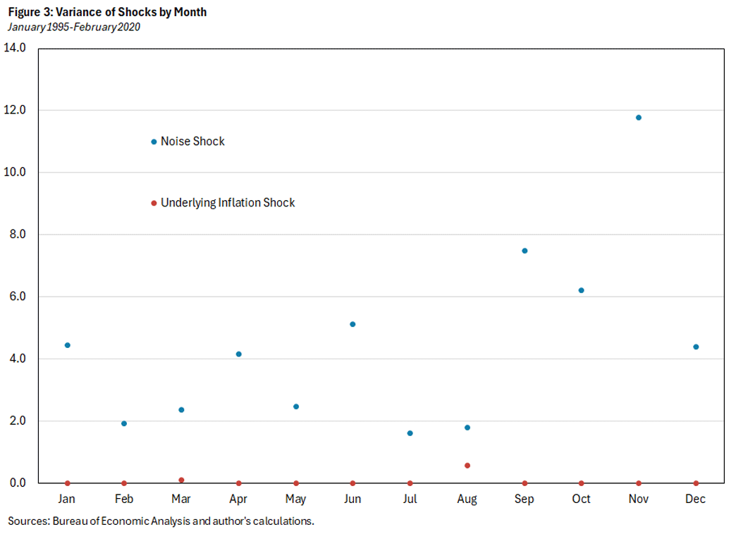
To summarize the difference between the two sets of variances, we can compare their respective mean and variance: Across months, the variance of the noise has a mean of 4.5 and variance of 8.8, whereas the variance of the underlying inflation shock has a mean of 0.06 and a variance of 0.03.

Implications

There are large differences across months in the estimated variances of the two shocks to the inflation process. Do these differences have economically important implications? We answer this question in two ways:

• First, we show how a fixed-size inflation surprise changes our beliefs about underlying inflation depending on the month.
• Second, we show how our estimate of the evolution of underlying inflation is affected by allowing for month-specific variances.

According to our statistical model, the optimal one-month-ahead forecast of the inflation rate is equal to the previous-month estimate of underlying inflation. We refer to the "inflation surprise" as the difference between the current inflation rate and the previous month's estimate of underlying inflation. That inflation surprise, in turn, leads to a revision in our estimate of underlying inflation.

For example, if we thought last month that underlying inflation was 2.0 percent and then observed inflation this month of 3.0 percent, we would move up our estimate of underlying inflation. But how much would we move it? The answer depends on the month-by-month variances of the noise and the shock to underlying inflation.

This is easier to understand when the variances do not differ by month: If the noise shock has high variance and the underlying inflation shock has low variance, then inflation surprises will generally be attributed to noise and will lead to only small revisions in our estimate of underlying inflation.

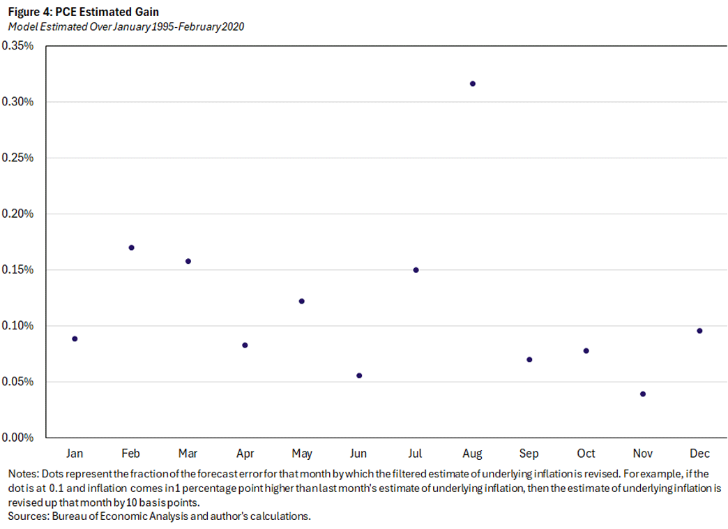
Figure 4 plots the "gain" for each month. The gain is the amount by which we adjust our estimates of underlying inflation in response to surprises, as just described. If the variances did not differ across month, then the gain would be the same for each month. In fact (and not surprisingly), there is large variation across months: The average gain is 0.12, with a low of 0.04 for November and a high of 0.32 for August. In other words, an inflation surprise of 1 percentage point would push up our estimate of underlying inflation by 0.04 percentage points in November and by 0.32 percentage points in August.

We now turn to the behavior of underlying inflation over time. Based on our model, there are two versions of underlying inflation that are interesting to look at, referred to as "filtered" and "smoothed." Filtered inflation follows directly from the above discussion of gain: We begin in January 1995 with an assumed level of underlying inflation of 2 percent, then update that level each period based on the surprise and the gain. Filtered inflation is a "one-sided" estimate: For a given month, it is calculated using only data up to that month.

In contrast, smoothed inflation is a "two-sided" estimate: Each month's estimate is based on the entire sample of data.⁶ Whereas filtered inflation is calculated by moving forward one period at a time, smoothed inflation works backward, starting from the last filtered estimate. It updates going backward in time, based on the difference between the current period's smoothed estimate and the previous period's filtered estimate. Intuitively, if the current period's smoothed estimate of underlying inflation is lower than the previous period's filtered estimate, then smoothing will push down the previous period's estimate. Not surprisingly, smoothed inflation is much smoother than filtered inflation.

Figure 5 plots the smoothed estimate of underlying inflation and the estimate from a restricted version of the model where there is no seasonality in variance.⁷ The chief difference between these estimates is that the restricted version is much smoother. Evidently, allowing for seasonality in variance is important for capturing the variation in underlying inflation. The most recent estimate shows a lower value of underlying inflation for the preferred unrestricted model: 2.87 percent compared to 3.16 percent.

Focusing now on the preferred model that allows for seasonality in variance, Figure 6 plots both the filtered and smoothed estimates of underlying inflation. As expected, filtered underlying inflation is more volatile than its smoothed counterpart. The current estimate of underlying inflation is 2.87 percent (based on data through February 2025). The February inflation rate was 4.01 percent, whereas the predicted value based on data through January was 2.65 percent — necessarily equal to the estimate for (filtered) underlying inflation in January. Multiplying the February gain of 0.17 from Figure 4 by the inflation surprise of 1.36 percentage points explains why the estimate of underlying inflation moved up from 2.65 percent to 2.87 percent. It is notable that the smoothed estimate of underlying inflation has moved up about 0.25 percentage points since August 2024.

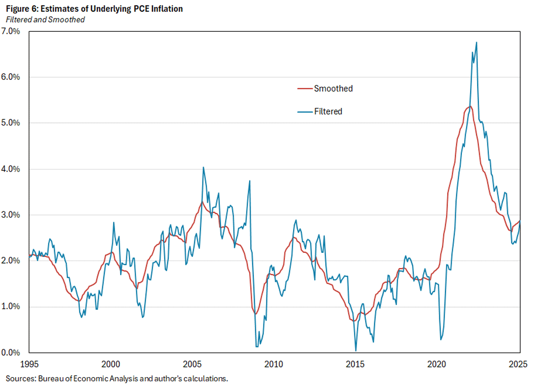
Figure 7 zooms in on the COVID and post-COVID periods, showing the month-by-month revisions to filtered underlying inflation together with the corresponding inflation surprises. We choose to display filtered instead of smoothed underlying inflation in Figure 7 to illustrate the near-real-time evolution of estimated underlying inflation according to our model.⁸

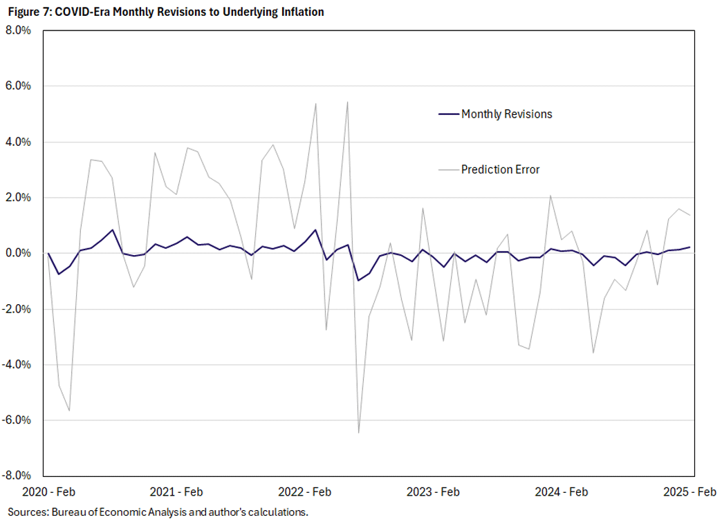
From December 2020 through March 2022, inflation surprised to the upside in all but one month. Thus, underlying inflation moved up in all but one month. July 2022 marked a turning point: An inflation overprediction of 6.4 percentage points — combined with the July gain of 0.15 percentage points — caused our estimate of underlying inflation to move down by almost a full percentage point. In the restricted version of the model where variances are constant across months (which is not shown in the figure), the July 2022 inflation rate was also greatly overpredicted. However, this led estimated underlying inflation to fall by only 0.26 percentage points.

In the subsequent 31 months ending in February 2025, our preferred model has overpredicted inflation in 19 of those months, leading to large downward movements in the estimated level of underlying inflation. Recent months, however, have seen some modest reversal of that progress.

Alexander L. Wolman is a vice president in the Research Department of the Federal Reserve Bank of Richmond. The author thanks Paul Ho and Felipe Schwartzman for helpful conversations.

To cite this Economic Brief, please use the following format: Wolman, Alexander L. (April 2025) "How Seasonality in Inflation Variance Affects Estimates of Underlying Inflation." Federal Reserve Bank of Richmond Economic Brief, No. 25-14.

This article may be photocopied or reprinted in its entirety. Please credit the author, source, and the Federal Reserve Bank of Richmond and include the italicized statement below.

Views expressed in this article are those of the author and not necessarily those of the Federal Reserve Bank of Richmond or the Federal Reserve System.