A Model-Based Perspective on Inflation and the Distribution of Relative Price Changes

A series of articles starting in 2022 has discussed the empirical relationship between inflation and the distribution of relative price changes: In the stable regime from 1995 until the pandemic era, the monthly inflation rate was closely related to a measure of asymmetry or skewness in the distribution of relative price changes. In this article, we describe related research that uses a dynamic macroeconomic model to study how inflation is jointly determined by monetary policy and "relative price shocks," as well as other shocks.¹ We use that model to help us understand the factors that lead to the relationship emphasized in previous articles.

The Empirical Relationship Between Inflation and the Distribution of Relative Price Changes

Macroeconomics has a long tradition of viewing large price changes for particular categories of goods and services as especially important in determining the inflation rate over short periods. This thinking underlies the popularity of core inflation and (more recently) trimmed mean inflation:

• Core inflation removes the contribution of food and energy — which usually are categories with high volatility of price changes — from the inflation rate.
• Trimmed mean inflation removes a fixed share of categories, those with the highest and lowest price changes (with the categories varying across periods).

Instead of focusing on one of these alternate measures of inflation as a way of controlling for large price changes, we look at a statistic from the distribution of relative price changes. Before explaining the statistic, we need to provide some basic information about the distribution of relative price changes.

For any category of good or service, the nominal price change is the change in the dollar price of that item. The relative price change is the change in the "goods" price of that item, where the goods price means the price of the item relative to the price of the overall consumption basket.² Because the change in the nominal price of the overall consumption basket is the inflation rate — and the inflation rate is also the average nominal price change — it follows that the average relative price change is zero every month.

The fact that the average relative price change is zero has a notable implication for the distribution of relative price changes. In each month, we can split the distribution of relative price changes into positive and negative changes:

• The positive changes are for the items whose nominal price changes are greater than the inflation rate.
• The negative changes are for the items whose nominal price changes are less than the inflation rate.

If the expenditure share of items with positive relative price changes is very large (close to 1), then it must be that the average of those positive relative price changes is small compared to the average of the very small share of relative price decreases. If this were not the case, the relative price changes as a whole could not average out to zero.

To summarize: By the definition of relative price changes, the average relative price change must be zero. And because the average relative price change is zero, there is a tight relationship between the share of expenditures with relative price increases and the average size of relative price increases compared to the average size of the relative price decreases. That relationship says that the higher the share of relative price increases, the lower the ratio of the average relative price increase to the average relative price decrease.

How the Share of Relative Price Increases Can Help Us Understand Inflation

How is this useful? We began by talking about the potential role of large price changes in accounting for monthly inflation rates. The second property of the relative price change distribution suggests that the share of relative price increases in a given month could be a good summary statistic for the role of large price changes in a given month. And to the extent these large price changes are important for inflation, then the summary statistic may be useful for understanding inflation.

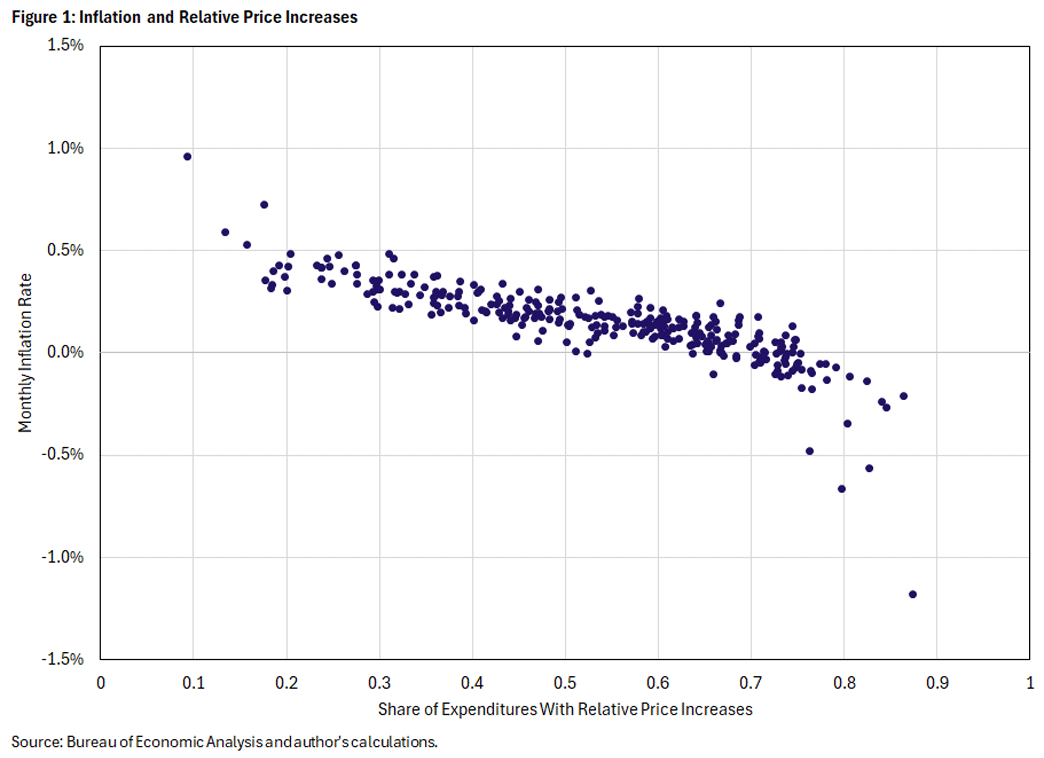
Figure 1 bears out this logic. The scatterplot comprises dots representing monthly data from January 1995 to February 2020. The vertical axis is the monthly inflation rate (measured in percent), and the horizontal axis is the monthly share of expenditures with relative price increases (nominal price increases that are greater than that month's inflation rate).³ When the share of relative price increases is high, the inflation rate tends to be low. And we know from properties of the relative price change distribution that these are months when the average relative price increase is much smaller than the (absolute value of the) average relative price decrease.

It's important to emphasize that Figure 1 covers a period when inflation and the monetary policy regime were generally stable. Over periods when those stability conditions do not hold, it would be surprising if a tight relationship exists like in Figure 1.

In previous articles, we used the relationship in Figure 1 as a benchmark against which to interpret data from the pandemic/postpandemic period beginning in March 2020.⁴ To the extent that high inflation readings were consistent with the prepandemic relationship to the share of relative price increases, they were less worrisome than a generalized upward shift in the relationship. In this article, we concentrate on the prepandemic relationship and interpret it through the lens of an economic model.

Description of the Macroeconomic Model

It may seem obvious that large price changes would be important for determining the inflation rate, but this is not a foregone conclusion in many standard macroeconomic models. To see this, we only need to note that it is feasible for monetary policy to perfectly stabilize the inflation rate in those models.⁵ If monetary policy can perfectly stabilize inflation regardless of the shocks to demand and supply for different categories of goods and services, then it follows directly that inflation can be unrelated to the distribution of relative price changes. Although the relationship in Figure 1 does not necessarily arise in a macroeconomic model, because it is present in the data it ought to be present in the models we use for policy analysis. In a particular model, one can then ask what features are important for replicating the empirical relationship.

We proceed in this manner. In economics jargon, our model is a multisector New Keynesian model. There are 15 categories of consumption goods and services, and the producers of those items face a cost to adjusting their prices. This means that prices do not instantaneously adjust fully to shocks, and it generates a role for monetary policy. Monetary policy is characterized by a so-called "Taylor rule," which sets the short-term interest rate as a function of inflation and output. The model's policy rule also includes interest rate smoothing, which means that the interest rate only partially adjusts toward its Taylor-rule target each period. An important feature of the model for matching the data is the rich set of sectoral shocks: In each sector, there are shocks that affect both the supply and demand for that sector's output.

What Features of the Model Are Important for Matching the Relationship?

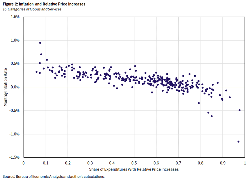
We estimate the model by maximum likelihood, using U.S. data on prices and quantities for 15 categories of consumption. Because these categories are broader than the 206 subcategories used to plot Figure 1, Figure 2 plots the analogous relationship based on 15 categories. It is of course not identical, but it shares the same broad properties as Figure 1.

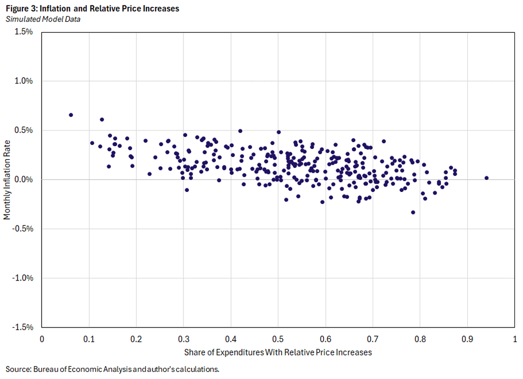
In Figure 3, we plot simulated data from the model, using the estimated parameters. That is, we simulate the model for the same number of months as plotted from the data, and for each month we plot the inflation rate against the share of expenditures for which the relative price increased in that month. The simulated data has fewer observations close to zero and 1, but the relationship between inflation and the monthly share of relative price increases is similar in the model and in the data.

Next, we investigate what features of the model are important for generating this relationship. In the 1995 paper "Relative Price Changes as Aggregate Supply Shocks," Laurence Ball and Gregory Mankiw brought attention to the relationship between inflation and the distribution of relative price changes. Using data from a period when inflation was not stable, they argued that inflation was related to interaction between shocks to the distribution of relative price changes and frictions in price setting. If firms faced fixed costs of price adjustment, then price adjustment will occur disproportionately from firms with large desired relative price adjustments. Thus, the distribution of desired relative price adjustments will affect the observed inflation rate.

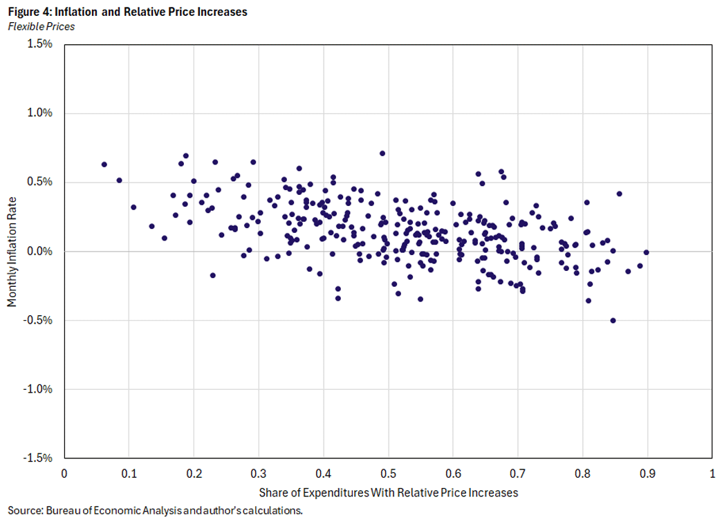
Our model does not include fixed costs of price adjustment, so its ability to match the relationship in Figure 1 must lie elsewhere. In Figures 4-7, we display the same scatterplot from simulated data for versions of the model in which specific sets of parameters are changed while the rest are held fixed at their estimated values. In this manner, we hone in on the crucial feature of the model that allows it to be consistent with the observed relationship between inflation and the distribution of relative price changes.

To begin, Figure 4 plots simulated data from a version of the model in which all prices are flexible. In the estimated model, there are separate price stickiness parameters in each sector and the estimates feature large variation in this parameter across sectors. Some research has suggested that differential price stickiness across sectors can be important for models' behavior, so we might expect that making price stickiness common across sectors by shutting it down entirely would have a large effect. In fact, Figure 4 shows that the effect is small: With flexible prices, there is little change to the relationship between inflation and the share of relative price increases.

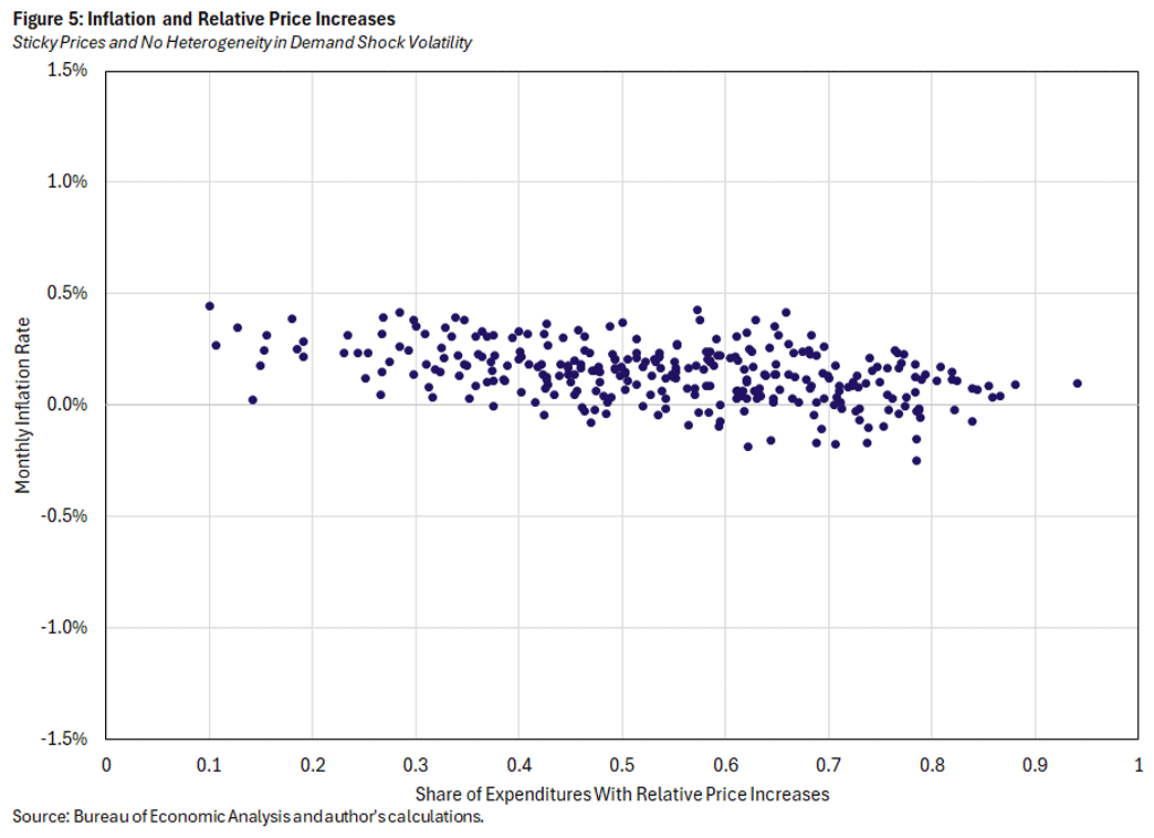
Next, we restore the estimated price stickiness parameters and shut down variation in demand shock volatility across sectors in Figure 5. There are still sector-specific demand shocks, but they are all drawn from the same distribution.

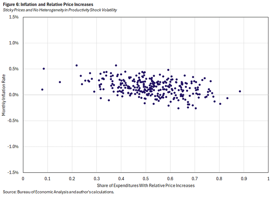
Analogously, we shut down variation in productivity shock volatility in Figure 6. While there are differences between figures 5 and 6 — inflation is less volatile with common demand shock volatility — the overall patterns in both cases are not much different from Figure 3.

We have now ruled out three aspects of the model as being necessary ingredients to generate the negative relationship between inflation and the share of relative price increases. Because that relationship involves heterogeneity across sectors, it must be that it comes about from some combination of the inherent heterogeneity across sectors with the way the model "processes" that heterogeneity and spits out an inflation rate.

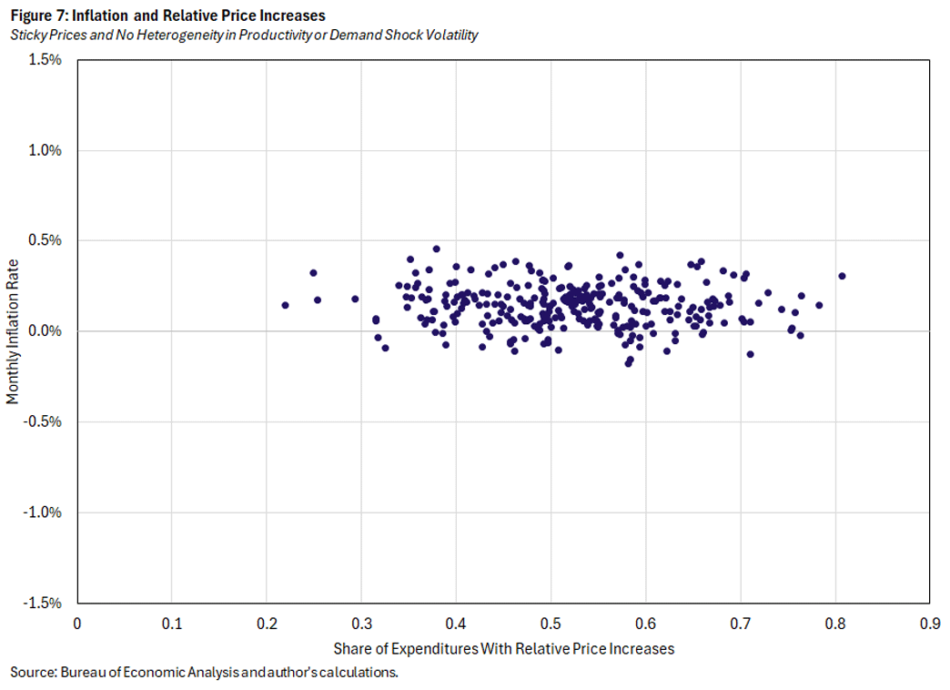
For Figure 7, we take up one of the few remaining aspects of inherent heterogeneity: We combine elements of Figures 5 and 6 by making demand-shock heterogeneity as well as productivity-shock heterogeneity common across sectors. And this does the trick: There is virtually no relationship between inflation and the share of relative price increases, as the correlation between the two variables is -0.06 in Figure 7, compared to -0.48, -0.47, -0.43 and -0.38 in Figures 3-6, respectively.

Heterogeneity in sectoral shock volatility, either for demand or productivity, is necessary for generating the negative empirical relationship between inflation and the share of relative price increases in our model. When shock volatility is identical across sectors, there is little opportunity for the kind of large idiosyncratic price changes that could meaningfully affect inflation. Large price changes could occur, but they would likely be met by offsetting price changes in the opposite direction. In contrast, with heterogeneity across sectors, the large price changes typically come from sectors with high volatility, and thus will not be met by offsetting price changes from other sectors. This helps to explain why it is necessary for volatility to differ across sectors to replicate the empirical relationship.

However, from the perspective of the model, it is not sufficient that there be heterogeneous volatility. As mentioned above, the relationship depends not only on sectoral heterogeneity but also on how the model processes that heterogeneity. And the most important feature of the model for that processing is monetary policy. From the standpoint of the model, monetary policy chooses to allow unusually large relative price changes for particular sectors to pass through to inflation, instead of responding in a way that generates large enough offsetting nominal price changes for all other categories to leave inflation unaffected.

Francisco Ruge-Murcia is a professor of economics at McGill University. Alexander L. Wolman is a vice president in the Research Department of the Federal Reserve Bank of Richmond.

To cite this Economic Brief, please use the following format: Wolman, Alexander L.; and Ruge-Murcia, Francisco. (September 2024) "A Model-Based Perspective on Inflation and the Distribution of Relative Price Changes." Federal Reserve Bank of Richmond Economic Brief, No. 24-30.

This article may be photocopied or reprinted in its entirety. Please credit the authors, source, and the Federal Reserve Bank of Richmond and include the italicized statement below.

Views expressed in this article are those of the authors and not necessarily those of the Federal Reserve Bank of Richmond or the Federal Reserve System.