Examining the Differences in r* Estimates

With inflation declining over the course of the year and the Federal Open Market Committee (FOMC) seemingly in the process of normalizing policy, a key question is: What is the natural real rate of interest (denoted r*)? In this article, we will shed light on what r* means, what models are used to estimate it and what the benefits and drawbacks are for these models.

This concept of the natural rate of interest was first developed by economist Knut Wicksell in 1898 as the interest rate compatible with a stable price level in the absence of any shocks or further disturbances to the economy. If the real policy rate is above r*, then policy can be considered restrictive. Normalization would imply bringing the policy rate down so that the real rate eventually coincides with r*. The real policy rate is connected to the nominal policy rate — the federal funds rate — by adding the inflation target rate of 2 percent to the real rate. In the context of current FOMC policy, the long-run federal funds rate is currently at 2.9 percent as projected in the September Summary of Economic Projections, while the current target range is 4.50 percent to 4.75 percent. A proper calibration of the policy stance therefore requires knowledge of r*.

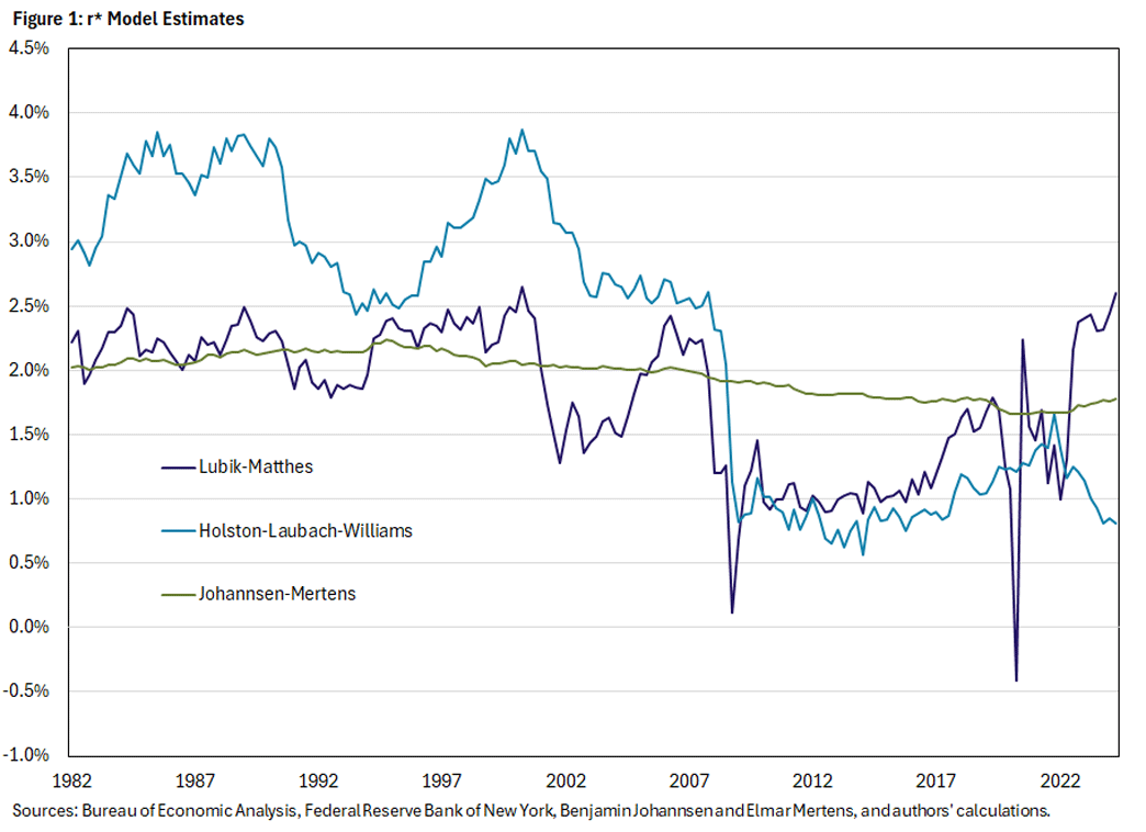
The challenge for policymakers is that r* cannot be measured directly from the data. As such, economists have developed a range of models to estimate r* using observed data. We show three leading estimates in Figure 1.

The wide range of estimates is striking in terms of both their levels and how volatile they are. For instance, the three estimates are 2.6 percent, 0.8 percent and 1.8 percent for the second quarter of 2024.

This presents a conundrum for policymakers: Which of these is most reliable? And how should one act in the face of uncertainty about which model to choose?

Lubik-Matthes: A Flexible Fully Statistical Model

The Federal Reserve Bank of Richmond regularly publishes one of these estimates: the Lubik-Matthes Natural Rate of Interest. This r* estimate is based on an article by one of the authors of this Economic Brief (Thomas) and Christian Matthes. The approach defines r* as the five-year-ahead forecast of the real interest rate based on a flexible statistical model. Over this long horizon, one would expect that the effect of many temporary disturbances will fade. The model forecast thus coincides with the real rate that the economy tends to converge toward in the absence of any additional disturbances, going back to the original definition of the natural rate in Wicksell's analysis.

The flexibility of the model is a key feature of the approach. Not only are there minimal restrictions placed on how the variables co-move, but the volatility of the data and relationships across variables are allowed to vary over time. For example, this allows the model to adapt to the unprecedented fluctuations in the data at the onset of the pandemic in 2020.

At the same time, the Lubik-Matthes model is purely statistical and nonstructural in the sense that the estimates are not easily connected to underlying economic relationships as described by macroeconomic theories. Moreover, its specification still forces the researcher to take a stance on how flexible the model is allowed to be. This requires the occasional recalibration of the model.

Holston-Laubach-Williams: Going Beyond the Data

A prominent alternative approach to estimating r* is the Holston-Laubach-Williams model. This model was developed by economists Kathryn Holston, Thomas Laubach and John Williams, and it is updated regularly by the Federal Reserve Bank of New York. The model uses more restrictions from economic theory and more closely resembles the macroeconomic models used by many central banks for policy analysis while still maintaining a good measure of statistical flexibility. The underlying equations are based on how GDP, inflation and interest rates interact in a workhorse class of macroeconomic models. Thus, it provides substantially more structure on how r* should move with the data than the Lubik-Matthes model.

The economic structure allows one to interpret r* in the model as the interest rate that is consistent with output when it is at its potential, which on average is consistent with the long-run productivity growth of the economy and stable inflation. This provides more of an economic (rather than statistical) interpretation of r*, unlike the Lubik-Matthes five-year-ahead forecast definition.

In principle, using a theoretical macroeconomic model in the estimation of r* adds information and therefore may yield a better estimate. However, the additional structure can be a double-edged sword in that it also potentially adds to the gap between model and data: All macroeconomic models are simplifications of the complex web of interactions in the economy. To match the data, the Holston-Laubach-Williams model includes processes not directly observed in the data, with some processes also lacking an interpretation consistent with the underlying economic model. Their behavior could reflect an attempt to estimate a model whose restrictions do not exactly match the data.

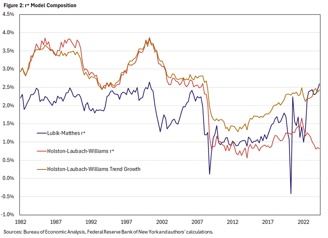
Specifically, r* in the Holston-Laubach-Williams model is explicitly defined as consisting of two components: trend productivity growth and a residual process. Figure 2 shows how this decomposition accounts for the recent gap between the Lubik-Matthes and Holston-Laubach-Williams r* estimates. Prior to 2005, the difference was primarily explained by the trend growth in the Holston-Laubach-Williams model, as it accounted for most of the variation in r*. In contrast, much of the recent gap is driven by the residual process, as the Lubik-Matthes r* is relatively close to the Holston-Laubach-Williams estimate of trend growth.

The connection with productivity growth follows from general economic reasoning. When trend productivity growth increases, r* should increase since firms expect greater returns to investments and are thus willing to pay higher rates of interest. For instance, firms might want to invest more to take advantage of expected future productivity gains from the development of AI. Higher productivity of capital is therefore closely linked to higher real interest rates.

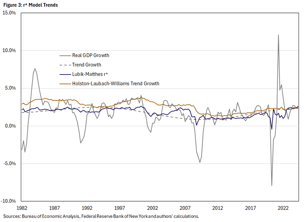
Importantly, trend productivity growth can be inferred directly from long-run GDP growth, but the model places additional restrictions on how it co-moves with GDP, inflation and interest rates. Figure 3 shows that the Holston-Laubach-Williams estimated trend growth lies above a 25-year trend of real GDP growth per capita estimated without further model restrictions, especially prior to 2010. In contrast, the Lubik-Matthes r* tracks the 25-year trend as predicted by theory, even though the Lubik-Matthes model does not explicitly impose such a relationship.¹

The residual process in the Holston-Laubach-Williams model likely captures features of the economic environment that are not included in the model and thus have no direct counterpart in the data. For instance, demographics or fiscal variables could be important determinants of the natural rate of interest.

In Figure 2, the residual process is simply the difference between the Holston-Laubach-Williams r* and trend productivity growth estimates. It remained around -0.4 percent through 2005 before subsequently declining. Crucially, 2023 saw a particularly sharp decline, coinciding with the divergence between the Lubik-Matthes and Holston-Laubach-Williams r* estimates. Recent work at the Federal Reserve Board of Governors has proposed the convenience yield attached to U.S. Treasuries as one explanation for these recent patterns. This describes the idea that debt issued by the U.S. government carries a lower interest rate than government debt from other developed countries because it is the world's safest security for foreign governments, banks and investors. This premium has arguably been rising over the last several decades in line with lower rates of return on account of this convenience yield. However, this pattern does not fully account for the earlier behavior of the residual process in the Holston-Laubach-Williams estimation.

Johannsen-Mertens: What Is Persistent?

An alternative way to trade off flexibility with restrictiveness lies in imposing minimal economic structure but explicitly distinguishing between temporary and permanent movements in the real interest rate and other macroeconomic variables. The permanent component of the real interest rate can then be interpreted as r*. Economists Benjamin Johannsen and Elmar Mertens have implemented such a specification in their 2021 paper "A Time-Series Model of Interest Rates With the Effective Lower Bound."

However, the Johannsen-Mertens estimate of r* is substantially more stable than the two alternative estimates above, remaining between 1.7 percent and 2.2 percent over the sample, as seen in Figure 1. Should one then infer that the natural rate has not moved much over the past 40 years?

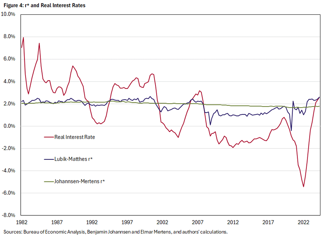
The answer depends on how r* is defined as an empirical concept and how economists can distinguish between transitory and persistent movements in the real rate. While the Lubik-Matthes r* represents a five-year-ahead forecast, the Johannsen-Mertens r* is the model's forecast of the real rate in the infinite future. Therefore, the Lubik-Matthes r* incorporates the effect of shocks that are persistent. That is, they still retain an effect after five years, even if they are not completely permanent. Figure 4 shows that this distinction was not important until after the Great Recession in 2007, when the real interest rate remained persistently low over a 12-year period.

The Johannsen-Mertens model allows a large degree of flexibility in the transitory component. In contrast, the economic structure of the Holston-Laubach-Williams model constrains transitory movements in the model variables, even though r* also corresponds to a permanent component of the real interest rate. As a result, the model assigns a greater share of the data fluctuations to the transitory component, leaving the permanent component (and hence r*) more stable. More generally, r* would tend to vary more over time in models that allow relatively less flexibility for temporary fluctuations as compared to persistent ones.

A New Hope?

The goal of the analysis above is not to advocate for any one approach over the others. In fact, policymakers do not need to choose any one estimate. Instead, a careful comparison of the approaches allows policymakers to discern possible strengths and weaknesses of each approach. Moreover, acknowledging the range of estimates also provides a sense of the uncertainty that policymakers need to consider.

Therefore, some informed judgement is required in deriving policy recommendations from model estimates of r*. Delving into the details of a model can provide hints of whether it overstates or understates the level of r*.

In addition, one should acknowledge the uncertainty by constantly learning from the incoming data. As interest rates fall, the response of prices and real variables can suggest how loose or tight monetary policy is. However, because such movements take time to occur, it is nevertheless helpful to have a broad sense of where r* is or how it might be moving. Furthermore, the models help policymakers form more coherent interpretations of the data evolution, thus informing future policy.

Paul Ho is a senior economist and Thomas A. Lubik is a senior advisor in the Research Department at the Federal Reserve Bank of Richmond.

To cite this Economic Brief, please use the following format: Lubik, Thomas A.; and Ho, Paul. (November 2024) "Examining the Differences in r* Estimates." Federal Reserve Bank of Richmond Economic Brief, No. 24-36.

This article may be photocopied or reprinted in its entirety. Please credit the authors, source, and the Federal Reserve Bank of Richmond and include the italicized statement below.

Views expressed in this article are those of the authors and not necessarily those of the Federal Reserve Bank of Richmond or the Federal Reserve System.